Lecture 7

Continuous Random Variables

Grace Tompkins

Last modified — 21 Jun 2026

Learning Outcomes

By the end of this lecture, students are anticipated to be able to:

Define a continuous random variable
Define and identify a probability density function
Define, identify, and apply common families of continuous distributions

1 Continuous Random Variables

Continuous Random Variables

A RV \(X\) is continuous if \[\mathbb{P}(X=x) = 0,\] for every \(x\in{\mathbb{R}}\).

This is the most rigorous way to define continuous RVs, but it doesn’t provide much intuition.
We need a bit more to make our intuition match the math.

Absolutely Continuous RVs and Density Functions

A function \(f : {\mathbb{R}}\to {\mathbb{R}}\) is called a density function if \(f(x)\geq 0,\ \forall x\in{\mathbb{R}}\) and \(\int f(x)\mathsf{d}x=1\).

A RV \(X\) is absolutely continuous if there exists a density function \(f\) such that \[\mathbb{P}(a\leq X\leq b) = \int_a^b f(x)\mathsf{d}x\] whenever \(a\leq b\).

We call such a density function a probability density function (PDF) and will often use the notation \(f_X(x)\) to denote its relationship to \(X\).

Absolutely Continuous RVs

Let \(X\) be an absolutely continuous random variable. Then \(X\) is a continuous random variable (i.e., \(\mathbb{P}(X = a) = 0\) for all \(a \in {\mathbb{R}}\))

\(\mathbb{P}(X = a) = \mathbb{P}(a \le X \le a) = \int_a^a f(x) dx = 0\)

Note

Note: the converse is not necessarily true. That is, not all continuous distributions you will come across in statistics (in general) are absolutely continuous. We will stick to absolutely continuous distributions in this course.

Comparison to Discrete RVs

Consider some set \(A \subset {\mathbb{R}}\).
Let \(X\) be a random variable.

Probability of \(A\) for discrete RV:

\[\mathbb{P}(X \in A) = \sum_{x \in A} p_X(x).\]

Probability of \(A\) for an (absolutely) continuous RV:

\[\mathbb{P}(X \in A) = \int_{A} f_X(x) \mathsf{d}x.\]

Example

Let \(X\) be a RV with PDF \[f_X(x) = 2 x^{-3} I_{[1,\infty)}(x).\]

Is \(X\) absolutely continuous? What is \(f_X(2)\)?
What is \(\mathbb{P}(0<X<2)\)?
Suppose we defined \(g(x) = 2 x^{-3}\) (no indicator function). Is \(g(x)\) a density function? Does is have the same support?

Example

2 Continuous families

(Continuous) Uniform

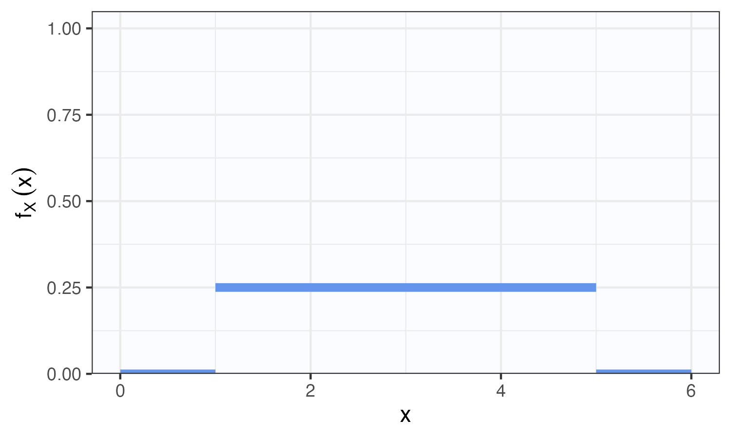
Let \(L < R \in {\mathbb{R}}\). A RV \(X\) with PDF \[f_X(x; L, R) = \frac{1}{R-L}I_{[L,R]}(x),\] is said to have the \({\mathrm{Unif}}(L,R)\) distribution.

\[ \begin{aligned} \mathbb{P}(a< X < b) &= \frac{1}{R-L}\int_a^b I_{[L,R]}(x) \\ &= \frac{b-a}{R-L}, \end{aligned} \] whenever \(L\leq a<b\leq R\).

Continuous Uniform Median

For continuous random variables, the median is the number \(m\) such that \[\mathbb{P}(X<m) = \mathbb{P}(X>m) = 1/2.\]

Let \(X\sim{\mathrm{Unif}}(L, R)\). What is the median of \(X\)?

Continuous Uniform Median

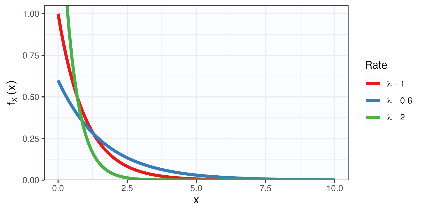
Exponential Distribution

Let \(\lambda>0\). A RV \(X\) with PDF \[f_X(x; \lambda) = \lambda e^{-\lambda x}I_{[0,\infty)}(x),\] is said to have the \({\mathrm{Exp}}(\lambda)\) distribution with rate \(\lambda\).

Exponential Distribution

\[f_X(x; \lambda) = \lambda e^{-\lambda x}I_{[0,\infty)}(x)\]

Let \(Y \sim {\mathrm{Exp}}(2)\). Find \(\mathbb{P}(Y > y)\) for \(y>0\).

Exponential Distribution

A small coffee shop receives customers independently at an average rate of 12 per hour. Let \(T\) be the waiting time (in minutes) between consecutive customer arrivals.

What distribution does \(T\) follow, and what is its rate parameter \(\lambda\)?
What is the probability that the next customer arrives within 3 minutes?

Exponential Distribution

Gamma Distribution

Recall the gamma function:

\[ \Gamma(\alpha) = \int_0^\infty t^{\alpha-1}\exp(-t)dt, \text{. where } \alpha > 0 \]

Useful results:

\(\Gamma(\alpha + 1) = \alpha\Gamma(\alpha)\)
If \(\alpha\) is an integer, this integral simplifies to \(\Gamma(n) = (n-1)!\)
\(\Gamma(1/2) = \sqrt(\pi)\)

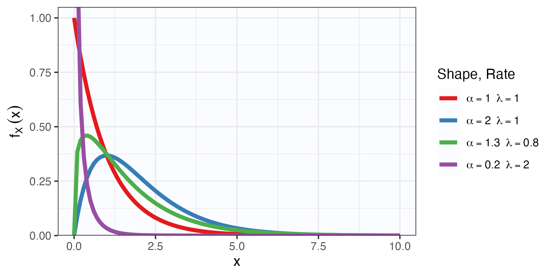
Gamma Distribution

Let \(\alpha, \lambda>0\). A RV \(Z\) with pdf \[f_Z(z; \alpha, \lambda) = \frac{\lambda^\alpha}{\Gamma(\alpha)} z^{\alpha-1}e^{-\lambda z}I_{[0,\infty)}(z),\] is said to have the \({\mathrm{Gam}}(\alpha,\lambda)\) distribution with shape \(\alpha\) and rate \(\lambda\).

Note: \(Z\sim{\mathrm{Gam}}(1,\lambda) \Rightarrow Z\sim{\mathrm{Exp}}(\lambda)\).

Gamma Distribution

The time to process an insurance claim follows \({\mathrm{Gam}}(\alpha = 2, \lambda = 1/3)\). What is the probability that the claim takes more than 6 hours to process?

Gamma Distribution

Kernel and Integration Constant

\[ \begin{aligned} f_Z(z; \alpha, \lambda) &= \frac{\lambda^\alpha}{\Gamma(\alpha)} z^{\alpha-1}e^{-\lambda z} I_{[0,\infty)}(z). \end{aligned} \]

PDFs/PMFs must integrate/sum to 1.
The functional form can be thought of as two pieces:
1. The “kernel” is the portion that depends on the argument (\(x\) or \(z\))
2. The “normalizing constant” is the part that depends only on parameters; this makes the function integrate to 1.
The support (given by the indicator function) is part of the kernel.

Kernel and Integration Constant: Example

\[f_Z(z; \alpha, \lambda) = \frac{\lambda^\alpha}{\Gamma(\alpha)} z^{\alpha-1}e^{-\lambda z} I_{[0,\infty)}(z)\]

The kernel is \(z^{\alpha}e^{-\lambda z} I_{[0,\infty)}(z)\).
The normalizing constant is \(\lambda^\alpha / \Gamma(\alpha)\).

We know that \[1 = \int_0^\infty \frac{\lambda^\alpha}{\Gamma(\alpha)} z^{\alpha-1}e^{-\lambda z} \mathsf{d}z \Longrightarrow \frac{\Gamma(\alpha)}{\lambda^\alpha} = \int_0^\infty z^{\alpha-1}e^{-\lambda z} \mathsf{d}z.\]

Kernel Matching

\[f_Z(z; \alpha, \lambda) = \frac{\lambda^\alpha}{\Gamma(\alpha)} z^{\alpha-1}e^{-\lambda z} I_{[0,\infty)}(z)\]

What is \[\int_0^\infty z^3 e^{-5z} \mathsf{d}z?\]
What is \[\int_0^\infty z \frac{\lambda^4}{\Gamma(4)} z^{3}e^{-\lambda z} \mathsf{d}z?\]

Hint: Recall that \(\Gamma(n) = (n-1)!\) when \(n \in \{1,2,\dots\}\).

Kernel Matching

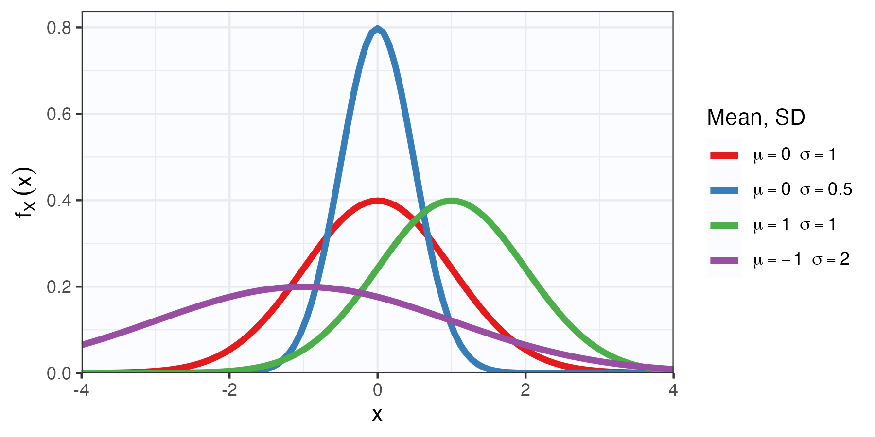
The Normal (Gaussian) distribution

Let \(\mu\in{\mathbb{R}}\), \(\sigma>0\). A RV \(Z\) with pdf \[f_Z(z; \mu, \sigma^2) = \frac{1}{\sqrt{2\pi\sigma^2}} \exp\left\{ -\frac{(z-\mu)^2}{2\sigma^2}\right\},\] is said to have the \(\mathcal{N}(\mu, \sigma^2)\) distribution.

The Normal Distribution

This distribution is incredibly important.
The reason is that it is good for modelling averages. We’ll justify this rigorously later.
\(Z \sim \mathcal{N}(0,1)\) is called the standard normal distribution. When \(Z\) is written without context, it is often understood to have this specific distribution.
Unfortunately \[\mathbb{P}(a<Z<b) = \int_a^b \frac{1}{\sqrt{2\pi}} e^{-z^2/ 2} \mathsf{d}z,\] does not have a closed form solution.
Old folks (like me) used tables in textbooks to calculate this (Table D.2 on p. 712 for you).
Nowadays, we use software.

To do:

Read Chapter 2.5 before next class
Assignment 2 due tomorrow, May 27th @ 11:59pm.
Midterm is next Tuesday during class.