Lecture 8

Cumulative Distribution Functions and Transformations

Grace Tompkins

Last modified — 21 Jun 2026

Learning Outcomes

By the end of this lecture, students are anticipated to be able to:

Define a cumulative distribution function (CDF)
Calculate CDFs from PDF/PMFs
Perform change of variables to calculate CDFs and PDFs/PMFs for functions of random variables.

1 Cumulative Distribution Functions (CDFs)

Cumulative Distribution Functions (CDFs)

The cumulative distribution function of a random variable \(X\) is \[F_X(x) \, = \, \mathbb{P}\left( X \le x \right) \, , \qquad \mbox{ for } x \in {\mathbb{R}}\]

Let \(X\) be a random variable with CDF \(F_X\). Then:

\(0 \le F_X(x) \le 1\) for all \(x \in {\mathbb{R}}\);
\(F\left( x \right) \leq F(y)\) for all \(x \leq y\);
\(\lim_{a \to -\infty} F_X\left( a \right) =0\),
\(\lim_{a \to +\infty} F_X\left( a \right) =1\)

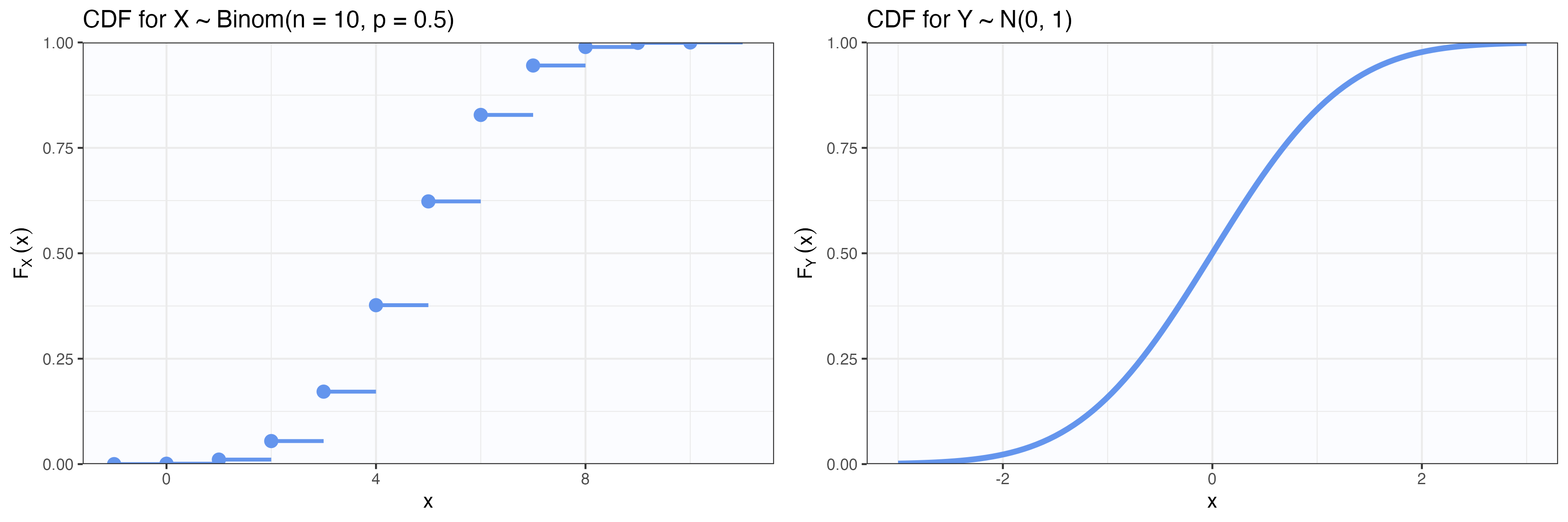
CDFs for Discrete and Continuous RVs

Discrete RV

\[F_X(x) = \sum_{t \leq x} p_X(t)\]

The CDF is a step function and right-continuous.

Continuous RV

\[F_X(x) = \int_{-\infty}^x f_X(t) \mathsf{d}t\]

The CDF is continuous (left and right limits are equal).

Continuous CDF Example

Let \(X \sim {\mathrm{Exp}}(\lambda)\), with pdf \[f_X(x) = \lambda e^{-\lambda x} I_{[0,\infty)}(x).\]

Find \(F_{X}\left(x \right)\). Use the CDF to calculate \(\mathbb{P}(x \le 10)\) when \(\lambda = 1/5\).

Continuous CDF Example

Discrete CDF Example

Consider rolling one fair six-sided die, so that \(\Omega = \{1, 2, 3, 4, 5, 6\}\), with \(\mathbb{P}(\omega) = 1/6\) for each \(\omega \in \Omega\) Let \(X\) be the number showing on the die. What is \(F_{X}(x)\)? Use this to find \(\mathbb{P}(X \le 5)\).

CDFs and Distributions

Let \(X\) be any random variable with CDF \(F_X\). Let \(B\) be any subset of \({\mathbb{R}}\). Then \(\mathbb{P}(X \in B)\) can be determined solely from \(F_X\).

The CDF contains all the information about the distribution of \(X\).
It doesn’t matter whether \(X\) is discrete, continuous, or anything else.

Let \(X\) be an absolutely continuous random variable with cumulative distribution function \(F_X\). Let

\[ f_X(x) = \frac{d}{dx}F_X(x) = F'(x). \] Then, \(f(x)\) is the density function for \(X\).

Aside: The discrete case involves finding the differences between consecutive CDF values.

Mixture Distributions

Let \(X_1, X_2,\dots\) be a random variables with CDFs \(F_{X_1}, F_{X_2}, \dots\).

For any constants \(p_i\) such that \(p_i \ge 0\) and \(\sum_{i = 1}^k p_i = 1\), \(F_G(x) = \sum_{i = 1}^k p_i F_{X_i}(x)\) is the CDF of the mixture of \(F_{X_i}\).

Mixture Distributions

Suppose a bag contains two coins. You choose one at random and flip it once. Let \(X\) be the number of heads.

Coin A is a fair coin, with \(\mathbb{P}(\text{flip Heads}) = 0.5\) Coin B is a loaded coin, with \(\mathbb{P}(\text{flip Heads}) = 0.9\)

Write out the CDF for the number of heads flipped.

Mixture Distributions

Consider the scores of a midterm. Suppose that there are three types of students, modeled as follows:

Poorly prepared students who did not study much (30%): \(X_1 \sim \mathcal{N}(\mu = 50, \sigma = 10)\).
Well prepared students who studied a lot (60%): \(X_2 \sim \mathcal{N}(\mu = 80, \sigma = 8)\).
Students who didn’t take the exam at all (10%): \(X_3 = 0\) with probability 1.

Find the CDF of the overall score distribution \(X\). Write your answer in terms of the standard normal CDF \(\Phi(\cdot)\).

Hint: If \(Y \sim \mathcal{N}(\mu, \sigma)\), then \(F_Y(y) = \Phi\left( \frac{y - \mu}{\sigma} \right)\).

Mixture Distributions

2 Transformations of CDFs

One-Dimensional Change of Variables

Sometimes we want to perform transformations on a random variable. This is when we can turn to change of variables.

Let \(X\) be a random variable with some distribution
Let \(Y = g(X)\) for some function \(g : {\mathbb{R}}\to {\mathbb{R}}\).
We want to find the distribution of \(Y\).

There are two ways to do this: the distribution method and the Jacobian method. We will present both.

One-Dimensional Change of Variables: Distribution Method

The distribution method just uses the definition:

\[\mathbb{P}(Y \in A) = \mathbb{P}(g(X) \in A) = \mathbb{P}(\{x : g(x) \in A\}).\]

If we can characterize these sets, we can find the distribution of \(Y\). This method always works, and is easy for discrete random variables.

Let \(X\) be a discrete random variable with PMF \(p_X(x)\). Let \(Y = g(X)\) for some function \(g : {\mathbb{R}}\to {\mathbb{R}}\). Then the PMF of \(Y\) is given by \[p_Y(y) = \sum_{x : g(x) = y} p_X(x) = \sum_{x \in g^{-1}(y)} p_X(x).\]

One-Dimensional Change of Variables: Distribution Method

Let’s make this method a little more algorithmic.

If you want to find the distribution of \(Y = g(X)\), then you can do the following: \[\mathbb{P}(Y \in A) = \mathbb{P}(g(X) \in A) = \mathbb{P}(\{x : g(x) \in A\}) = \cdots\]

Start with the definition of the distribution of \(Y\).
Use the definition of \(Y\) in terms of \(X\) to rewrite the probability in terms of \(X\).
Use the distribution of \(X\) to compute the probability that \(g(X) \in A\).
Then play algebra games to get it into a nice form; possibly “match” a known PDF or CDF.

One-Dimensional Change of Variables: Distribution Method (Discrete)

Let’s start with a straightforward example:

Let \(X \sim {\mathrm{Binom}}(n, \theta)\), for some \(\theta \in (0,1)\).
Let \(Y = n - X\).

Find the PMF of \(Y\).

One-Dimensional Change of Variables: Distribution Method (Discrete)

One-Dimensional Change of Variables: Distribution Method (Continuous)

Let \(X \sim {\mathrm{Exp}}(\lambda)\), find the distribution of \(Y = 3X\).

One-Dimensional Change of Variables: Distribution Method (Continuous)

If \(X \sim {\mathrm{Exp}}(\lambda)\), what is the CDF of \(Y = X + 5\)?

One-Dimensional Change of Variables: Useful Results

The following useful results follow from the previous examples

If \(X\) be a random variables with CDFs \(F_{X}\) Then the the following hold:

The RV \(Y = X + c\) has CDF \(F_{X}(x - c)\);
The RV \(Y = kX\) has CDF \(F_{X}(x/k)\) for any \(k > 0\);

One-Dimensional Change of Variables: Jacobian Method

For continuous random variables, you can also use the distribution method, and sometimes this is the easiest way. The other common method is the Jacobian method.

Let \(X\) be an (absolutely) continuous random variable, with density function \(f_X\). Let \(Y = h(X)\), where \(h : {\mathbb{R}}\to {\mathbb{R}}\) is a function that is differentiable and monotonic.

Then \(Y\) is also absolutely continuous, and its density function \(f_Y\) is given by \[f_Y(y) = f_X(h^{-1}(y)) \left| \frac{\mathsf{d}}{\mathsf{d}y} (h^{-1}(y)) \right|,\] where \(h^{-1}(y)\) is the unique number \(x\) such that \(h(x) = y\).

One-Dimensional Change of Variables: Jacobian Method

Let \(X \sim {\mathrm{Unif}}(0,1)\).
Let \(Y = -\log(X)\).

Find the PDF of \(Y\).

One-Dimensional Change of Variables: Jacobian Method

Let \(X \sim {\mathrm{Unif}}\left( -1,1\right)\). Use the distribution method to find the PDF of \(Z = X^2\).
Let \(X \sim {\mathrm{Gam}}(\alpha, \lambda)\). Use the Jacobian method to find the PDF of \(Y = 1/X\).

Recall the Gamma PDF: \[f_X(x) = \frac{\lambda^\alpha}{\Gamma(\alpha)} x^{\alpha - 1} e^{-\lambda x} I_{(0, \infty)}(x).\]

One-Dimensional Change of Variables: Jacobian Method

This is the end of the “testable” content for your midterm.

Your midterm will cover materials from Lectures 1 - 8
DATE: in class on Tuesday June 2
LENGTH: 1 hour and 50 minutes in length.
You may bring in one (1) “cheat sheet”:
- Must be HAND WRITTEN with pen/pencil on said sheet of paper (not typed, not photo copied, not printed, not written on an iPad)
- Must be on 8.5 by 11 inch sheet of paper or smaller
- You may write on both sides
- No magnifying glasses or anything else silly
- I will confiscate cheatsheets that do not follow these rules 🥀
- I do not care what is written on it
Exam is hand written on paper, bring something to write with
You may bring a non-programmable, non-graphing calculator.

To do:

Read Chapter 2.7 before next class
Assignment 2 due tonight, May 27th @ 11:59pm.
Start reviewing for your midterm. No assignment due next week.