Lecture 14

Conditional Expectations and Inequalities

Grace Tompkins

Last modified — 21 Jun 2026

Learning Outcomes

By the end of this lecture, students are anticipated to be able to:

• Calculate conditional expectations from conditional and joint distributions
• Use inequalities to find bounds of expectations and variances

1 Conditional Expectation

Conditional Expectation

If \(X\) and \(Y\) are two random variables, then the conditional expectation of \(X\) given \(Y = y\) is \[\begin{aligned} \mathbb{E}\left[ X | Y= y \right] &= \int_{-\infty }^{\infty } x f_{X|Y}\left( x | y \right) \mathsf{d}x, & \mathbb{E}\left[ X | Y= y \right] &= \sum_{x} x p_{X|Y}(x|y). \end{aligned}\]

• This is the same definition we saw previously for expectation, just with the conditional distribution.

Conditional Expectation

Let \(X\) and \(Y\) be random variables with joint density \(f(x, y) = 2\) for \(0 < x < 1, 0 < y < x\). What is the conditional expectation of \(Y\) given \(X\)?

Conditional Expectation

Conditional Variance

If \(X\) and \(Y\) are two random variables, then the conditional variance of \(X\) given \(Y = y\) is \[\begin{aligned} \operatorname{Var}(X | Y = y ) &= \int_{-\infty }^{\infty } ( x - \mathbb{E}[X|Y=y] ) ^{2}f_{X|Y}\left( x|y \right) \mathsf{d}x,\\ \operatorname{Var}(X | Y = y ) &= \sum_{x} ( x - \mathbb{E}[X|Y=y] ) ^{2}p_{X|Y}(x|y). \end{aligned}\]

Conditional Variance

Let \(X\) and \(Y\) be random variables with joint density \(f(x, y) = 2\) for \(0 < x < 1, 0 < y < x\). What is the conditional variance of \(Y\) given \(X\)?

Try this on your own.

Conditional Variance

Conditional Expectation and Variance

Sometimes we are directly given information about the conditional distribution. If this is a “known” distribution, we can just use the properties of that distribution.

• Let \(\Theta \sim {\mathrm{Unif}}(0, 1)\)
• Let \(Y | \Theta = \theta \sim {\mathrm{Binom}}(n, \theta)\)

What are \(\mathbb{E}[Y|\Theta=\theta]\) and \(\operatorname{Var}(Y|\Theta=\theta)\)?

Because the conditional expecation follows \({\mathrm{Binom}}(n, \theta)\), we know:

• \(\mathbb{E}[Y|\Theta=\theta] = n\theta\) and
• \(\operatorname{Var}(Y|\Theta=\theta) = n\theta(1-\theta)\).

This is much easier than finding the PMF/PDF of Y.

Conditional Expectation and Variance

Important

Quick knowledge check. Are conditional expectations and variances random variables?

Conditional Expectation and Variance

• The properties of expectation and variance that we have seen before also hold for conditional expectation and variance.

But there are some additional properties as well because \(\mathbb{E}[X|\Theta]\) and \(\operatorname{Var}[X|\Theta]\) are themselves random variables, and have their own distributions.

Let \(\Theta \sim {\mathrm{Unif}}(0, 1), \text{ and } Y | \Theta = \theta \sim {\mathrm{Binom}}(n, \theta)\)

• \(W = \mathbb{E}[Y|\Theta] = n\Theta\) is a random variable that depends on \(\Theta\).
• But \(\Theta \sim {\mathrm{Unif}}(0, 1)\), so \(W \sim {\mathrm{Unif}}(0, n)\)!
• Using the Jacobian method, we can show that the PDF of \(V = \operatorname{Var}(Y|\Theta) = n\Theta(1-\Theta)\) is given by \[f_V(v) = \frac{2}{n\sqrt{1 - 4v/n}}, \quad 0 < v < n/4.\]

Hierarchical Models

We refer to this general setup as a hierarchical model.

1. We first draw \(\Theta\) from some distribution.
2. Then we draw \(Y\) from a distribution that depends on \(\Theta\).
3. We can find the distribution of \(Y | \Theta\) as well as those of its expectation.

• Let \(\Lambda \sim {\mathrm{Gam}}(1, 2)\).
• Let \(X | \Lambda \sim {\mathrm{Exp}}(1/\Lambda)\).

Find the distribution of \(W = \mathbb{E}[X|\Lambda]\) and \(\mathbb{E}[W]\).

Hierarchical Models

Law of Total Expectation

Using the definition of the joint distribution of \(X\) and \(\Lambda\), we can show that \[\begin{aligned} f_{X,\Lambda}(x, \lambda) &= f_{X|\Lambda}(x|\lambda) f_{\Lambda}(\lambda) \\ &= \frac{1}{\lambda} e^{-x/\lambda} \cdot \frac{1}{\Gamma(1)} \lambda e^{-\lambda} I_{[0,\infty)}(x)I_{[0,\infty)}(\lambda) \\ &= e^{-x/\lambda}e^{-\lambda} I_{[0,\infty)}(x)I_{[0,\infty)}(\lambda). \end{aligned}\]

Using our definition of Expectation, we can find \(\mathbb{E}[X]\): \[\begin{aligned} \mathbb{E}[X] &= \int_0^\infty \int_0^\infty x e^{-x/\lambda}e^{-\lambda} I_{[0,\infty)}(x)I_{[0,\infty)}(\lambda) \mathsf{d}\lambda \mathsf{d}x = \cdots. \end{aligned}\]

That is: \[\mathbb{E}[X] = \mathbb{E}[W] = \mathbb{E}[\mathbb{E}[X|\Lambda]].\]

Law of Total Expectation and Variance (Tower Property)

Let \(X\) and \(Y\) be two random variables. Then, \[\mathbb{E}[X] = \mathbb{E}[\mathbb{E}[X|Y]]\] and \[\operatorname{Var}(X) = \mathbb{E}[\operatorname{Var}(X|Y)] + \operatorname{Var}(\mathbb{E}[X|Y]).\]

• The first equation shows what we just saw, but it is general and holds for any \(X\) and \(Y\).
• The second equation is a bit more complicated, but it is also very useful.
• It shows that the variance of \(X\) can be decomposed into two parts: the expected value of the conditional variance of \(X\) given \(Y\), and the variance of the conditional expectation of \(X\) given \(Y\).

Law of Total Expectation and Variance (Tower Property)

Let \(X\) and \(U\) be random variables such that \(U \sim Unif(0. 1)\), and \(\mathbb{E}[X\ \vert\ U] = 3U^2\). Find \(\mathbb{E}[X]\).

Law of Total Expectation and Variance (Tower Property)

2 Inequalities

Markov’s Inequality

Let \(X\) be a random variable with \(\mathbb{P}(X \geq 0) = 1\). Then, for any \(a > 0\), \[\mathbb{P}( X \geq a ) \le \frac{\mathbb{E}[ X ] }{a}.\]

Note that this implies that for any random variable \(Y\),

\[\mathbb{P}(|Y| \geq a) \le \mathbb{E}[|Y|] / a.\]

Proof of Markov’s Inequality

Let \(Z = a I_{[a,\infty)}(X)\). We have that \(Z \leq X\) almost surely, and hence \(\mathbb{E}[Z] \leq \mathbb{E}[X]\) by monotonicity of expectation. But \[\begin{aligned} \mathbb{E}[X] &\geq \mathbb{E}[Z]\\ &= a \mathbb{P}(Z = a) + 0 \mathbb{P}(Z = 0)\\ & = a \mathbb{P}(Z = a)\\ &= a\mathbb{P}(X \geq a). \end{aligned}\]

Chebyshev’s¹ Inequality

Let \(X\) be a random variable with finite mean \(\mu\).

Then, for any \(a > 0\), \[\mathbb{P}(| X - \mu| \geq a ) \leq \ \frac{\operatorname{Var}(X)}{a^2}.\]

1. Your book uses Chebychev, and many other transliterations of the name exist (e.g., Tchebychev, Tchebycheff, Čebyčev, Čebyšev, Chebysheff, Chebychov and Chebyshov). We will use Chebyshev, which is what the AMS uses.

Chebyshev’s¹ Inequality

We have \[\begin{aligned} \mathbb{P}( |X - \mu| \geq a) &=\mathbb{P}( (X - \mu) ^2 \geq a^2) \\ &\leq \frac{\mathbb{E}[(X - \mu) ^2 ] }{a^{2}} & \textrm{(by Markov's ineq.)}\\ &=\frac{\operatorname{Var}(X)}{a^{2}}. \end{aligned}\]

1. Your book uses Chebychev, and many other transliterations of the name exist (e.g., Tchebychev, Tchebycheff, Čebyčev, Čebyšev, Chebysheff, Chebychov and Chebyshov). We will use Chebyshev, which is what the AMS uses.

Comparing Markov and Chebyshev

Let \(X\) be a non-negative random variable with mean \(\mu\) and variance \(\mu\).

We want to examine the bounds on \(\mathbb{P}((X - \mu)/\mu \geq 1)\) given by Markov’s and Chebyshev’s inequalities.

Markov’s inequality gives \[\mathbb{P}((X - \mu)/\mu \geq 1) = \mathbb{P}( X \geq 2\mu ) \leq \ \frac{\mathbb{E}[X]}{2\mu} = \frac{\mu}{2\mu} = \frac{1}{2}.\]

Chebyshev’s inequality gives \[\mathbb{P}((X - \mu)/\mu \geq 1) = \mathbb{P}(X - \mu \geq \mu) \leq \mathbb{P}(|X - \mu| \geq \mu) \leq \frac{\operatorname{Var}(X)}{\mu^2} = \frac{\mu}{\mu^2} = \frac{1}{\mu}.\]

So for any random variable with mean \(\mu\) and variance \(\mu\), Chebyshev’s inequality gives a tighter bound whenever \(\mu > 2\).

Binomial Bounds

Suppose you flip a fair coin 100 times. Use Markov’s and Chebyshev’s inequalities to approximate the probability of seeing 60 or more heads.

Binomial Bounds

Far Away Stars

• Suppose that a radio telescope can measure the distance to a star.
• But due to atmospheric conditions, instrumental error, and movements of the earth, each measurement is a random variable with mean \(\mu\) light years (the true distance) and variance \(4\) (square) light years.
• An astronomer plans to take \(n\) independent measurements of the distance and use their average \(\overline{X}_n\) as an estimate for the true distance.

How many measurements should the astronomer make if they want the probability of a mismeasurement larger than 1 light year to be no more than 0.01?

Hint: recall that \(\mathbb{E}[ \overline{X}_n ] = \mathbb{E}[X_1]\) and \(\operatorname{Var}( \overline{X}_n ) = \operatorname{Var}(X_1)/n\).

Far Away Stars

Cauchy Schwarz Inequality

Cauchy Schwarz for random variables

Let \(X\) and \(Y\) be two random variables with finite second moments. Then, \[|\mathbb{E}[XY]| \leq \sqrt{\mathbb{E}[X^2] \,\mathbb{E}[Y^2]}.\]

Let \(X\) and \(Y\) be two random variables with finite second moments. Then, \[|\operatorname{Cov}(X, Y)| \leq \sqrt{\operatorname{Var}(X) \, \operatorname{Var}(Y)}.\]

If, in addition, \(\operatorname{Var}(X) > 0\) and \(\operatorname{Var}(Y) > 0\), then \[|\operatorname{Corr}(X, Y)| \leq 1.\]

Jensen’s Inequality

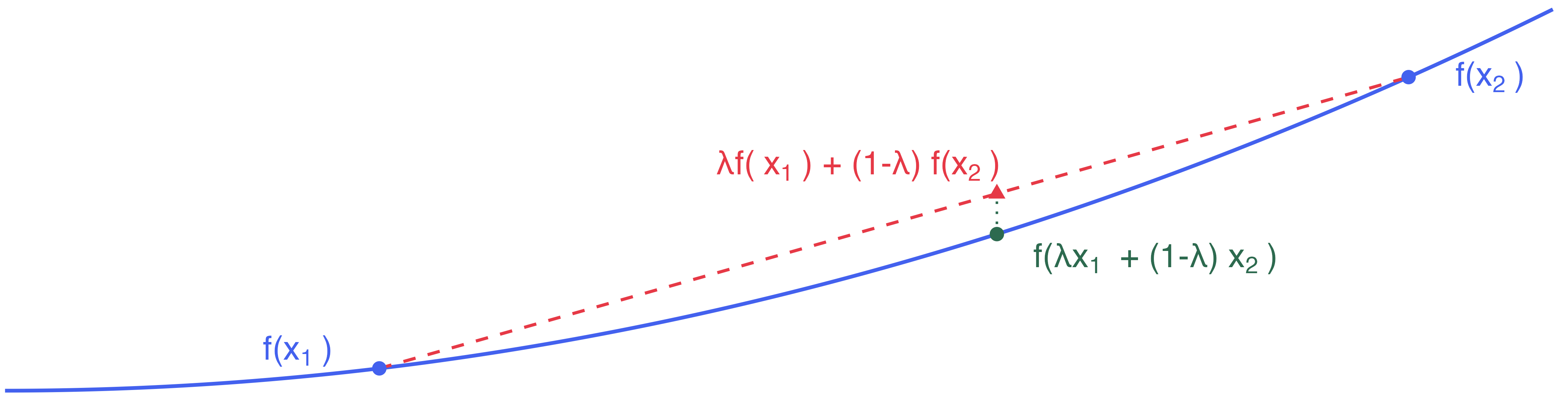
Recall that a function \(f: {\mathbb{R}}\to {\mathbb{R}}\) is convex if for any \(x, y \in {\mathbb{R}}\) and \(\lambda \in [0, 1]\), we have \[f(\lambda x + (1 - \lambda) y) \leq \lambda f(x) + (1 - \lambda) f(y).\]

Let \(X\) be a random variable with finite mean and let \(f: {\mathbb{R}}\to {\mathbb{R}}\) be a convex function. Then, \[f(\mathbb{E}[X]) \leq \mathbb{E}[f(X)].\]

Questionable Friendships

Your friend offers to play the following game with you.

1. Your friend pays you $49 to roll 2 standard 6-sided dice.
2. If you see \(x\) pips, you pay your friend $\(x^2\).
3. Repeat as many times as you like, and your friend will keep paying you $49 each time.

How many times should you play this game? Justify your answer.

Questionable Friendships

Followup on Jensen’s Inequality

Show that the variance of a random variable is always non-negative.

Followup on Jensen’s Inequality

To Do

• Work on Assignment 3, due TONIGHT June 10, 11:59pm on Gradescope.
• Read Chapter 4.2 - 4.3 before next class.