Lecture 16
Convergence, Part II
Grace Tompkins
Last modified — 21 Jun 2026
Learning Outcomes
By the end of this lecture, students are anticipated to be able to:
- Define convergence in distribution
- Determine when a sequence converges in distribution
- Define and apply the Central Limit Theorem (CLT)
1 Convergence in Distribution
Convergence in Distribution
A sequence of random variables \(X_1,X_2,\ldots,X_n,\ldots\) with CDFs \(F_n\) converges in distribution to a random variable \(X\) with CDF \(F\) if, for all \(t\) at which \(F\) is continuous, \[\lim_{n \to \infty} F_n(t) = F(t).\]
- We will see that this is the “weakest” notion of convergence.
- But it gets used more frequently than the others.
- Common notation: \(X_n \overset{d}{\to}X\).
If there exists \(s>0\) such that for all \(t \in (-s,s)\) \(m_{X_n}(t) \to m_X(t)\), then \(X_n \overset{d}{\to}X\).
Convergence in Distribution
Let \(U \sim {\mathrm{Unif}}(0,1)\), and let \(U_n\sim {\mathrm{Unif}}(0,1)\) all independent. Define
\[X_n = U_n + B_n\]
where \(B_n\sim {\mathrm{Bern}}(1/n)\) are independent Bernoullis, also independent of \(U, U_1, U_2, \ldots\).
Then \(X_n\overset{d}{\to}U\) but \(X_n\) does NOT converge in probability to \(U\).
We have that, for all \(t\), \[m_{X_n}(t) = m_{U_n}(t) m_{B_n}(t) = \frac{e^t - 1}{t} (1-\frac{1}{n} + \frac{1}{n}e^t) \to \frac{e^t - 1}{t} = m_U(t).\]
Convergence in Distribution
….continued….
However, \[\begin{aligned} \mathbb{P}(|X_n - U| > \epsilon) &= \mathbb{P}\left(|U_n + B_n - U| > \epsilon\right) \\ &= (1-1/n)\mathbb{P}\left(|U_n - U| > \epsilon\right) + (1/n)\mathbb{P}\left(|U_n +1- U| > \epsilon\right) \\ &= (1-1/n)(1-\epsilon)^2 + (1/n)a \quad\quad\text{for some $a\in[0,1]$}\\ &\rightarrow (1-\epsilon)^2 \neq 0. \end{aligned}\]
Convergence in Distribution
Let \(X_n\sim \mathcal{N}(0, 1 + 1/n)\) for all \(n\), mutually independent. Show that \(X_n \overset{d}{\to}Z\sim\mathcal{N}(0,1)\) by examining the moment generating functions.
Hint: Recall that the MGF of \(\mathcal{N}(\mu, \sigma^2)\) is \(m(t) = e^{\mu t + \sigma^2 t^2/2}\).
Convergence in Distribution
Course Evaluation
Please take 10 minutes to fill out the course evaluation. This will:
Help inform future course offerings (I’m teaching this again in Fall)
Provide feedback on my own teaching on where to improve
Help me stay employed in this economy :–)
I want you to fill this out regardless of how you feel about this course. Constructive feedback is welcome - rude comments about things I cannot change are not welcome. Keep it honest but professional - thank you!

Relationships Between Different Types of Convergence
The following implications hold for any sequence of random variables \(X_1, X_2, \ldots\) and any random variable \(X\): \[ X_n \overset{a.s.}{\to}X \Longrightarrow X_n \overset{p}{\to}X \Longrightarrow X_n \overset{d}{\to}X. \]
Interpreting convergence
- Convergence almost surely (with probability 1) is examining the sample path of \(X_n(\omega)\). We need this path to converge to the value of \(X(\omega)\) for almost all \(\omega\).
- Convergence in probability involves the joint distribution of \(X_n\) and \(X\): we are looking at the probability that \(|X_n - X|\) is small. We hope this probability goes to one.
- Convergence in distribution only involves the marginal distribution of \(X_n\). We are looking at the distribution of \(X_n\) and hoping it gets closer and closer to the distribution of \(X\) as \(n\) increases.
Visualization of Convergence
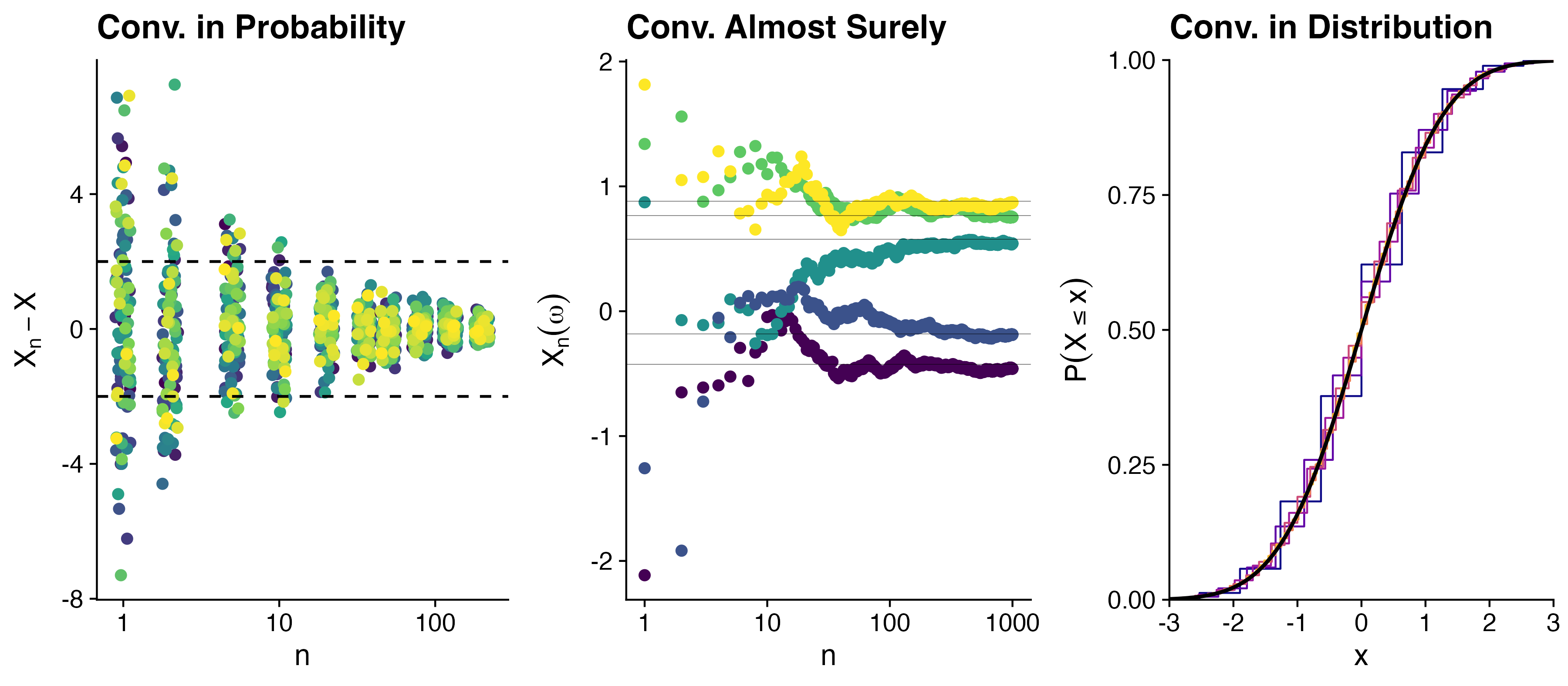
- The probability that \(X_n - X\) is large shrinks as \(n\) increases. (100 samples from \(X_n - X\))
- For each \(\omega\), the sample path \(X_n(\omega)\) gets closer and closer to \(X(\omega)\) as \(n\) increases.
- The CDF of \(X_n\) gets closer and closer to the CDF of \(X\) as \(n\) increases.
Convergence of Maximum of I.I.D Uniforms
Let \(U_1, U_2, \ldots\) be i.i.d. \({\mathrm{Unif}}(0,1)\) random variables. Define \(Y_n = \max\{U_1, \ldots, U_n\}\).
Show that \(n(1-Y_n) \overset{d}{\to}{\mathrm{Exp}}(1)\).
Hints:
Start by finding the CDF \(F_{Y_n}(t)\) of \(n(1-Y_n)\).
Recall that the CDF of \({\mathrm{Exp}}(1)\) is \(F(t) = 1 - e^{-t}\).
Convergence of Maximum of I.I.D Uniforms
Convergence in Probability vs Distribution
Let \(X_n\sim \mathcal{N}(0, 1 + 1/n)\), mutually independent, for all \(n\). Does \(X_n \overset{p}{\to}Z\sim\mathcal{N}(0,1)\)? Justify your answer.
2 Central Limit Theorem (CLT)
The Central Limit Theorem (CLT)
Let \(X_{1},X_{2}, \dots, X_n,\ldots\) be i.i.d random variables with finite mean \(\mu\) and variance \(\sigma^2\).
Then, \[ \frac{\sqrt{n}(\overline{X}_n-\mu )}{\sigma } \overset{d}{\to}\mathcal{N}\left( 0,1\right). \]
- People often say that \(\overline{X}_n\) converges to a standard Gaussian.
- They mean that \(\overline{X}_n\) appropriately normalized converges.
Interpretation
Probability statements about \(\overline{X}_n\) can be approximated using a Normal distribution. It’s the probability statements that we are approximating, not the random variable itself.
Equivalent Statements of the CLT
Define \[Z_n = \frac{\sqrt{n}(\overline{X}_n-\mu )}{\sigma }.\]
- There are several forms of notation that all basically say the same thing. \[\begin{aligned} Z_n &\approx \mathcal{N}(0,1)\\ \overline{X}_n &\approx \mathcal{N}\left(\mu, \frac{\sigma^2}{n}\right)\\ \overline{X}_n - \mu &\approx \mathcal{N}\left(0, \frac{\sigma^2}{n}\right)\\ \sqrt{n}(\overline{X}_n - \mu) &\approx \mathcal{N}(0, \sigma^2)\\ \frac{\overline{X}_n - \mu}{\sigma/\sqrt{n}} &\approx \mathcal{N}(0,1). \end{aligned}\]
Equivalent Statements of the CLT
You should not say things like:
\[\overline{X}_n \overset{d}{\to}\mathcal{N}(\mu, \sigma^2/n).\]
- This grosses me out because you are taking a limit on the left-hand side where \(n\) goes to infinity, but the distribution on the right-hand side still depends on \(n\).
Usefulness of the CLT
In many situations, the exact distribution of \(\overline{X}_n\), \(\mathbb{P}(\overline X_n \leq x)\), is hard to determine exactly.
The CLT allows us to approximate this value by
\[\mathbb{P}(\overline X_n \leq x) \approx \Phi\Big ( \frac{\sqrt{n}(x-\mu)}{\sigma}\Big )\] with a respectable precision when \(n\) is large.
- Some people say that this approximation has acceptable precision when \(n \ge 30\).
- Ignore those people.
- It would be more accurate to say “if \(n<30\), this approximation is probably bad”.
Far Away Stars, Revisited
- Suppose that a radio telescope can measure the distance to a star.
- But due to atmospheric conditions, instrumental error, and movements of the earth, each measurement is a random variable with mean \(\mu\) light years (the true distance) and variance \(4\) (square) light years.
- An astronomer plans to take \(n\) independent measurements of the distance and use their average \(\overline{X}_n\) as an estimate for the true distance.
Use the CLT to determine how many measurements the astronomer should make if they want the probability of a mismeasurement larger than 1 light year to be no more than 0.01?
Far Away Stars, Revisited
Far Away Stars, Discussion
Chebyshev’s inequality suggests \[n \ge 400\] independent observations.
CLT suggests \[n \ge 27\] independent observations
Both are correct, but the CLT is more precise.
To be fair, it used more information (the asymptotic distribution of the sample mean), which may or may not be accurate.
Chebyshev’s doesn’t use any approximation, it’s a guarantee.
Proof of the CLT
Let \(Z_n = \frac{\sqrt{n}(\overline{X}_n-\mu )}{\sigma}\) as before.
Define \(Y_i = (X_i - \mu)/\sigma\) for all \(i\).
- Then, \(Y_1, Y_2, \ldots\) are i.i.d. with mean \(0\) and variance \(1\), and we have \(\frac{1}{\sqrt{n}}\sum_{i=1}^n Y_i = Z_n.\)
- By the proposition about MGFs, we need to show that \(m_{Z_n}(t) \to m_Z(t)\) for all \(t,\) where \(Z\sim \mathcal{N}(0,1)\).
Suppose that \(Y_i\) has moment generating function \(m_Y(t)\).
- Then, the moment generating function of \(\sum Y_i\) is \(m_Y(t)^n\).
Therefore, the moment generating function of \(Z_n\) is \(m_Y(t/\sqrt{n})^n\).
Proof of the CLT, continued
Now, \(m'_Y(0) = \mathbb{E}[Y_i] = 0\) and \(m''_Y(0) = \mathbb{E}[Y_i^2] = 1\).
By Taylor’s theorem, for all \(t\), \[\begin{aligned} m_Y(t) &= m_Y(0) + m'_Y(0)t + \frac{1}{2}m''_Y(0)t^2 + \cdots\\ &= 1 + 0 + \frac{t^2}{2} + \frac{t^3}{3!}m'''_Y(0) + \cdots \\ &= 1 + \frac{t^2}{2} + \frac{t^3}{3!}m'''_Y(0)+ \cdots.\\ \Longrightarrow \quad m_{Z_n}(t) &= m_Y(t/\sqrt{n})^n \ = \left(1 + \frac{\frac{t^2}{2} + \frac{t^3}{3!n^{1/2}}m'''_Y(0) + \cdots}{n}\right)^n \to e^{t^2/2} = m_Z(t). \end{aligned}\]
[We used the fact that \(\lim_{n \to \infty} (1 + a_n/n)^n = e^a\) when \(a_n \to a\).]
Central Limit Theorem for I.I.D Sums
The CLT states that when \(n\) is large, the distribution of \[\frac{\overline{X}_n - \mu }{\sigma /\sqrt{n}} \text{ \ \ is \ approximately \ } \mathcal{N}\left( 0,1\right).\]
This implies that when \(n\) is large, we can also say something about the distribution of \(S_n = \sum_{i=1}^{n}X_{i}\).
\[\begin{aligned} 1-\Phi(z) &= \lim_{n\rightarrow\infty}\mathbb{P}\left( \frac{\overline X_n - \mu} {\sigma/\sqrt{n}} > z \right)\\ &=\lim_{n\rightarrow\infty}\mathbb{P}\left( \frac{(n\overline X_n - n\mu)} {n\sigma/\sqrt{n}} > z \right)\\ &=\lim_{n\rightarrow\infty}\mathbb{P}\left( \frac{S_n - n\mu} {\sqrt{n}\sigma} > z \right) \end{aligned}\]
Struggling Restaurants
The daily sales on any given day of a restaurant is a random variable with mean of $2500 and standard deviation of $500.
Assume that daily sales are independent random variables.
Give an approximate value of the probability that the total sale for the 30 days will be over $80,000.
Leave your answer in terms of \(\Phi\) (the CDF of a standard Gaussian).
Exam Prep Advice
- Review class slides and create a first draft of your cheat sheet first.
- Review in class exercises, midterm, and assignments before attempting these problems.
- Try out these Exam Prep Problems unassisted before looking at the answer.
- It is very easy to get a false sense of confidence if you look at the answer first! See how far you can get in the solution and allow yourself to get it wrong the first time.
- If you’re stuck, look for similar past questions and try to connect them.
- Look at the solution after giving the problem a genuine attempt.
- Consider adding/removing from your cheat sheet after trying these problems!
- Familiarize yourself with the distributions provided on the exam (see above), and your own cheat sheet.
- Ask for help if a solution is unclear. Piazza and office hours are resources that are here to help you.
Exam Rules
- The final exam is scheduled for Monday June 22nd at 8:30am. You can find the room location on Workday.
- It is 2 hours and 30 minutes and covers all content. There are 10 questions of similar length and difficulty to the midterm.
- You may bring in one (1) “cheat sheet”:
- Must be HAND WRITTEN with pen/pencil on said sheet of paper (not typed, not photo copied, not printed, not written on an iPad)
- Must be on 8.5 by 11 inch sheet of paper or smaller d
- You may write on both sides
- I will confiscate cheatsheets that do not follow these rules 🥀
- Bring a non-programmable, non-graphing calculator.
The final page of your exam will also contain common distributions and general mean/variances (download the sheet here)
To Do
- Work on Assignment 4, due Wednesday June 17, 11:59pm on Gradescope.
- Next class: Review session! Let me know what you want to review by leaving a reply on the Piazza thread.
Stat 302 - Winter 2025/26