Module 05

Families of random variables

TC and DJM

Last modified — 04 Feb 2026

Review of Random Variables

A random variable is a function that maps from the sample space to \({\mathbb{R}}\).
Typically denoted by \(X\), \(Y\), \(Z\) (letters near the end of the alphabet)
The distribution of a random variable is the collection of probabilities associated with every subset of \({\mathbb{R}}\) (we ignore details).

Why is this useful?

Random variables will allow us to quit worrying about the sample space, and simply deal with the abstraction.
Any properties we learn about the distribution of the random variable apply to any sample space that could possibly be “modelled” with that Random Variable.
We can leave the world of dice and coins and just talk about math.

We start with Discrete random variables.

1 Discrete random variables

Discrete random variables

Definition

We say that a random variable \(X\) is discrete if there exists a countable set \(K = \{x_1,x_2,\dots\}\) such that

\[\mathbb{P}(X \in K) = 1.\]

In particular, this means that \(\{x : P(X=x)>0\}\) is countable:

I can count the \(x\) that have positive probability.

For discrete RVs, we call the set \(\{x : P(X=x) > 0\}\) the support of \(X\). We may use the notation \(\operatorname{supp}(X)\).
These are the types of RV’s we’ve worked with so far. We’ll visit the other extreme next week.

Examples of experiments described by discrete random variables

Toss a fair coin 3 times, count the total number of Heads.
Roll a 6-sided die until you see 6, count the number of rolls.
Count the number of people that arrive at the bus stop in some amount of time.
Will it be rainy (\(-6\)), cloudy (2), or sunny (\(+10\)) on campus today?

Probability (mass) function (PMF)

For discrete random variables, we can be explicit about the probability associated with each value in it’s support

Definition

For a discrete random variable, its probability (mass) function is the function \(p_X : {\mathbb{R}}\rightarrow [0,1]\) defined by \[p_X(x) = \mathbb{P}(X = x).\]

It is occasionally written \(f_X(x) = \mathbb{P}(X = x).\)

Each of the examples of discrete random variables has a PMF. Once we write it down, we know everything there is to know.

Worked example

Suppose it rains 30% of the time, is cloudy but not raining 30%, and sunny 40% of the time.

Your happiness is given by the random variable \(Z\) with \(Z=-6, 2,\) and 10 respectively.

What is the support of \(Z\)?
What is the PMF of \(Z\)?

Your turn

Exercise 1

Toss a fair coin 3 times. Let \(X\) be the number of heads.

What is the support of \(X\)?
What is the \(p_X(x)\)?

Finding probabilities of events

The PMF can be used to find the probabilities of events.

We have that for some event \(A\) and a RV \(X\),

\[\mathbb{P}(X \in A) = \sum_{x \in A} p_X(x).\]

Let \(A\) be the event that you are happier than 0. Find \(\mathbb{P}(Z \in A)\).

Another PMF

For a fixed number \(\theta \in [0, 1]\), define a discrete random variable \(X\) with PMF given by:

\[ p_X\left( x;\ \theta\right) =\begin{cases} \left( 1-\theta\right) ^{2} & x=0, \\ 2\theta\left( 1-\theta\right) & x=1, \\ \theta^{2} & x=2, \\ 0 & \mbox{else.} \end{cases} \]

Different values of \(\theta\) will give different PMFs.

\[ p_X\left( x;\ \theta = 0.1\right) =\begin{cases} 0.81 & x=0, \\ 0.18 & x=1, \\ 0.01 & x=2 \\ 0 & \mbox{else.} \end{cases} \]

By including a parameter \(\theta\), we are able to express many distributions (a family of distributions) with a single functional form.

Urn example

An urn contains \(n\) balls numbered \((1, 2, \ldots, n)\).
Randomly draw \(k\) balls \((1<k<n)\) without replacement.
Let \(Y\) represent the largest number among them.

Exercise 2

What is support of \(Y\)?
Find \(p_{Y}\left(y\right)\).

2 Discrete families

Bernoulli

An experiment with 2 outcomes (success/failure).

Definition

Suppose the probability of success is \(\theta \in [0,1]\). A RV \(X\) with PMF given by

\[p_X(x; \theta) = \theta^x(1-\theta)^{1-x}I_{\{0,1\}}(x),\]

is said to have the \({\mathrm{Bern}}(\theta)\) distribution.

If \(\theta = 0.5\), then we have our favourite fair-coin friend.
But we can let \(\theta\) be numbers other than 0.5.

Binomial

A sequence of \(n\) independent Bernoulli trials, each with the same probability of success.

Definition

Suppose the probability of success is \(\theta \in [0,1]\). A RV \(X\) with PMF given by

\[p_X(x; n, \theta) = \binom{n}{x} \theta^x (1-\theta)^{n-x}I_{\{0,1,\dots,n\}}(x),\]

is said to have the \({\mathrm{Binom}}(n, \theta)\) distribution.

We saw this earlier in the specific case of \(n=3\) coins, and \(\theta=0.5\).
It also applies the number of Wins for a bad (or good or middling) sports team.
Or if you repeatedly play backgammon against your significant other and count defeats.

Using the Binomial

\[p_X(x; n, \theta) = \binom{n}{x} \theta^x (1-\theta)^{n-x}I_{\{0,1,\dots,n\}}(x)\]

Exercise 3

Suppose Midterm 1 has 5 True/False questions. What is the probability that you get at least 4 correct answers by random guessing?
Suppose Midterm 1 has 2 multiple choice questions with 5 options. What is the probability that you get both correct by random guessing?

Poisson

Definition

A RV \(Y\) with PMF given by

\[p_Y(y; \lambda) = \frac{\lambda^y}{y!}e^{-\lambda} I_{\{0,1,2,\dots\}}(y),\]

is said to have the \({\mathrm{Poiss}}(\lambda)\) distribution.

Poisson is good for modelling counts of things, often per unit of time.
How many people come to the bus stop in 5 minutes?
How many purchases will be made of some item on Amazon in a day?
How many times does a neuron fire while you perform a task?

Poisson

This is not the only distribution that is good for modelling counts, and we’ll see reasons to choose a different one later.

Sometimes written \[p_Y(y; \lambda t) = \frac{(\lambda t)^y}{y!}e^{-(\lambda t)} I_{\{0,1,2,\dots\}}(y),\] where \(\lambda\) is “per unit time” and \(t\) is the number of seconds/minutes/days/etc.

Poisson maximization

Exercise 4

Suppose that \(Y\sim {\mathrm{Poiss}}(\lambda)\), and you observe \(Y=5\). What value of \(\lambda\) makes \(\mathbb{P}(Y=5)\) as large as possible?

\[p_Y(y; \lambda) = \frac{\lambda^y}{y!}e^{-\lambda} I_{\{0,1,2,\dots\}}(y)\]

Hint: Take the \(\log\)!

Other important (named) discrete distributions

\({\mathrm{Geom}}(\theta)\) — Flip a coin with \(\mathbb{P}(\text{success}) = \theta\) until you see the first success. How many flips?
\({\mathrm{NegBinom}}(r, \theta)\) — Flip a coin with \(\mathbb{P}(\text{success}) = \theta\) until you see \(r\) successes. How many flips?
\({\mathrm{HypGeom}}(N, M, n)\) — An urn with \(M\) red balls and \(N-M\) white balls. Draw \(n\) balls without replacement. How many are red?
\({\mathrm{Categorical}}(\{p_1,\dots,p_K\})\) — Generalization of \({\mathrm{Bern}}(\theta)\) to \(K\) outcomes instead of 2.
\({\mathrm{Multinom}}(n, \{p_1,\dots,p_K\})\) — Generalization of \({\mathrm{Binom}}(n, \theta)\) to \(K\) outcomes instead of 2.

For each of these (and many others), we don’t need to “count” stuff. We just ask the math formula (or software) to calculate the probabilities of outcomes.

The trick is to translate the word problem to the correct named distribution.

Translation

Exercise 5

For each of the following experiments, name the distribution that would make an appropriate model, and if obvious, identify the value(s) of any parameters.

How many fries can you throw at the seagulls on Granville Island before they eat six?
Roll a die until you see 6. How many rolls?
Given 1000 bank transactions, an auditor samples 50 to check for fraud. If all 50 are legitimate, what is the probability that the remainder contains fraud?
How many patients arrive at the ER in 3 hours?

3 Continuous random variables

Continuous random variables

Definition

A RV \(X\) is continuous if \[\mathbb{P}(X=x) = 0,\] for every \(x\in{\mathbb{R}}\).

This is the most rigorous way to define continuous RVs, but it doesn’t provide much intuition.
So while, \(\mathbb{P}(X=x)=0\), it will often be the case that for an open ball, \(B(x,\delta)\), of radius \(\delta>0\), \(\mathbb{P}(X\in B(x,\delta))>0\).
We need a bit more to make our intuition match the math.

Absolutely continuous RVs and density functions

Definition

A function \(f : {\mathbb{R}}\to {\mathbb{R}}\) is called a density function if \(f(x)\geq 0,\ \forall x\in{\mathbb{R}}\) and \(\int f(x)\mathsf{d}x=1\).

Definition

A RV \(X\) is absolutely continuous if there exists a density function \(f\) such that \[\mathbb{P}(a\leq X\leq b) = \int_a^b f(x)\mathsf{d}x\] whenever \(a\leq b\).

We call such a density function a probability density function (PDF) and will often use the notation \(f_X(x)\) to denote its relationship to \(X\).

Comparison to discrete RVs

Consider some set \(A \subset {\mathbb{R}}\).
Let \(X\) be a random variable.

Probability of \(A\) for discrete RV:

\[\mathbb{P}(X \in A) = \sum_{x \in A} p_X(x).\]

Probability of \(A\) for an (absolutely) continuous RV:

\[\mathbb{P}(X \in A) = \int_{A} f_X(x) \mathsf{d}x.\]

Comparison to discrete RVs

Support of discrete RV \(X\):

\[\operatorname{supp}(X) = \{x : \mathbb{P}(X=x) > 0\} \subset \{x : \sum_x \mathbb{P}(X=x) = 1\}.\]

Support of an (absolutely) continuous RV \(X\):

\[\operatorname{supp}(X) = \{x : \mathbb{P}(X \in B(x,r)) > 0,\ \forall r > 0 \} = \{x : f_X(x) > 0 \}.\]

It is the smallest set \(A\subseteq {\mathbb{R}}\) such that \(\mathbb{P}(X\in A) = 1\).

An example continuous RV

Exercise 6

Let \(X\) be a RV with PDF \[f_X(x) = 2 x^{-3} I_{[1,\infty)}.\]

Is \(X\) absolutely continuous? What is \(f_X(2)\)?
What is \(\mathbb{P}(0<X<2)\)?
Suppose we defined \(g(x) = 2 x^{-3}\) (no indicator function). Is \(g(x)\) a density function? Does is have the same support?

4 Continuous families

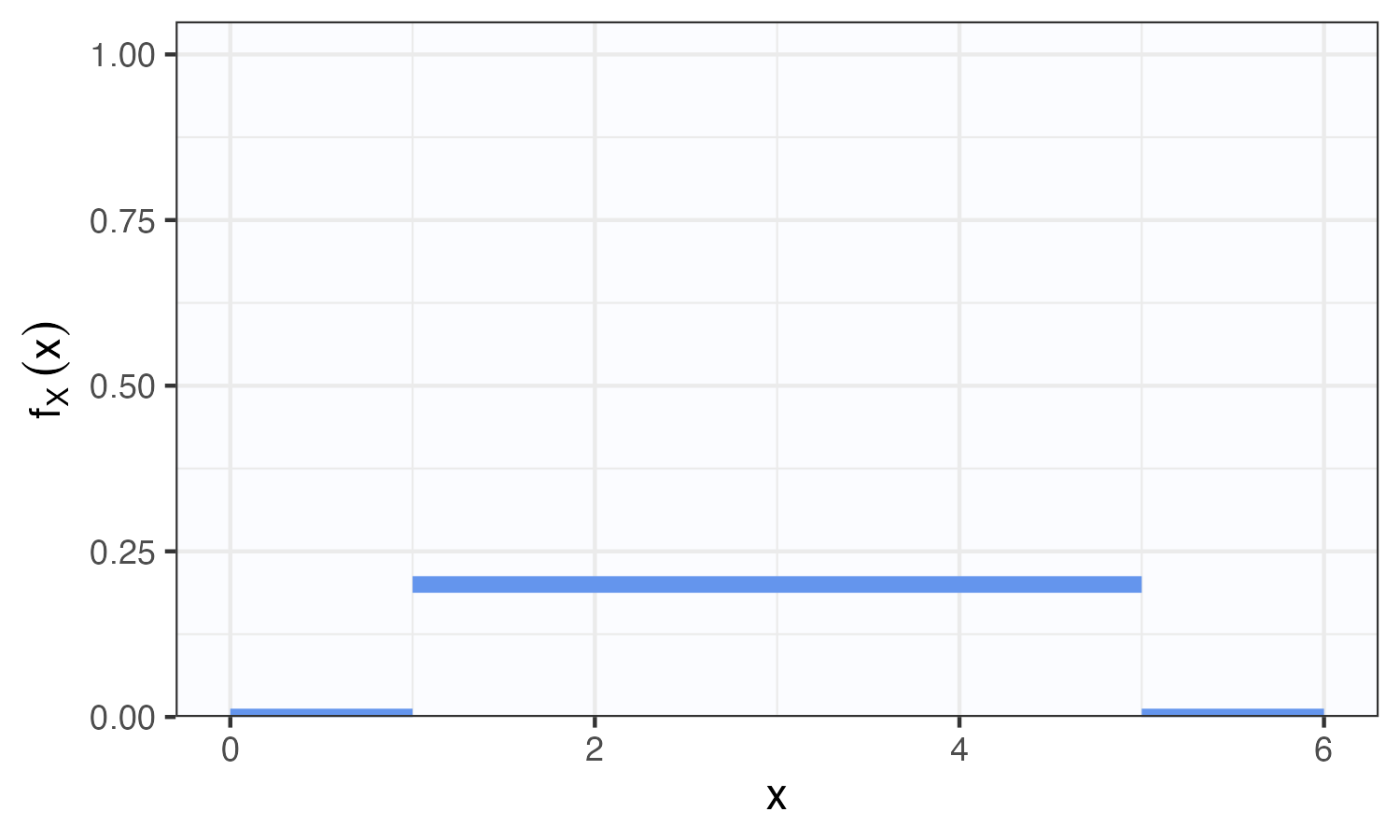
(continuous) Uniform

Definition

Let \(L < R \in {\mathbb{R}}\). A RV \(X\) with PDF \[f_X(x; L, R) = \frac{1}{R-L}I_{[L,R]}(x),\] is said to have the \({\mathrm{Unif}}(L,R)\) distribution.

\[\begin{aligned} \mathbb{P}(a< X < b) &= \frac{1}{R-L}\int_a^b I_{[L,R]}(x) \\ &= \frac{b-a}{R-L}, \end{aligned}\] whenever \(L\leq a<b\leq R\).

Uniform median

Exercise 7

For continuous random variables, the median is the number \(m\) such that \[\mathbb{P}(X<m) = \mathbb{P}(X>m) = 1/2.\]

Let \(X\sim{\mathrm{Unif}}(L, R)\). What is the median of \(X\)?

Exponential distribution

Definition

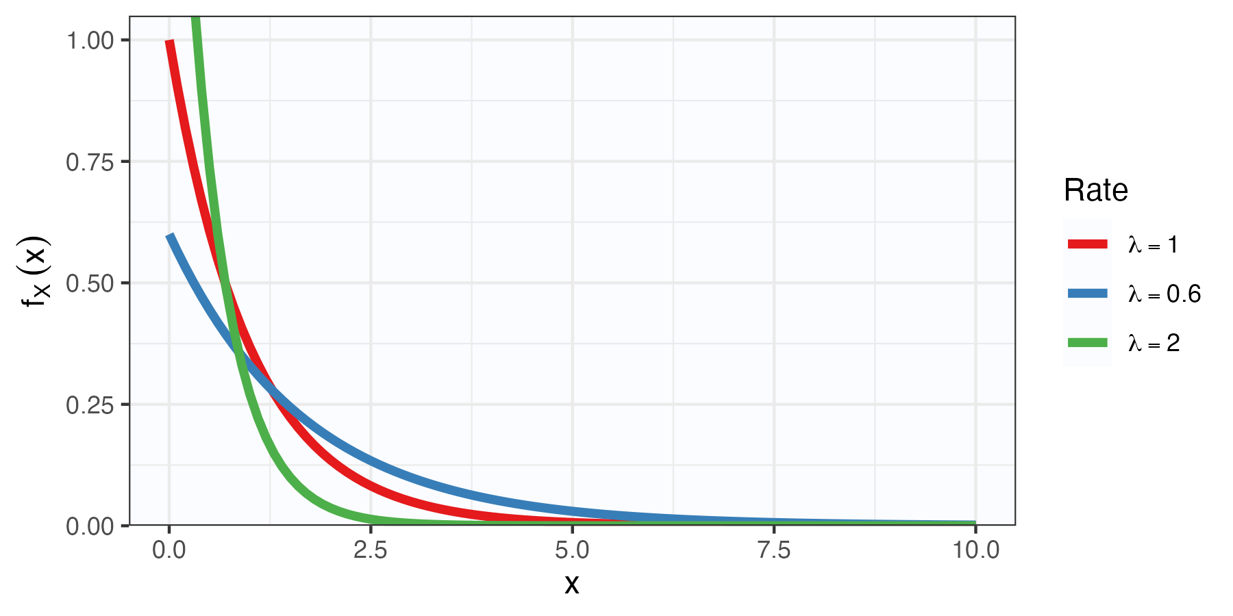
Let \(\lambda>0\). A RV \(X\) with PDF \[f_X(x; \lambda) = \lambda e^{-\lambda x}I_{[0,\infty)}(x),\] is said to have the \({\mathrm{Exp}}(\lambda)\) distribution with rate \(\lambda\).

Exponential distribution

\[f_X(x; \lambda) = \lambda e^{-\lambda x}I_{[0,\infty)}(x)\]

Exercise 8

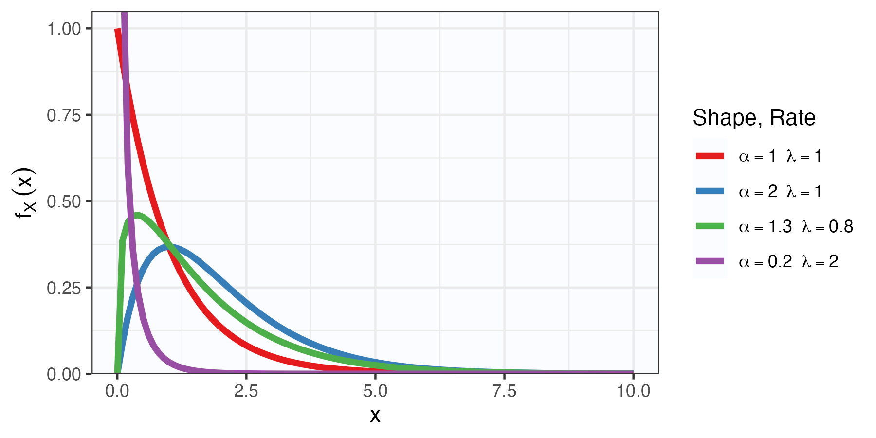
Let \(Y \sim {\mathrm{Exp}}(2)\). Find \(\mathbb{P}(Y > y)\) for \(y>0\).

Gamma distribution

Definition

Let \(\alpha, \lambda>0\). A RV \(Z\) with pdf \[f_Z(z; \alpha, \lambda) = \frac{\lambda^\alpha}{\Gamma(\alpha)} z^{\alpha-1}e^{-\lambda z}I_{[0,\infty)}(z),\] is said to have the \({\mathrm{Gam}}(\alpha,\lambda)\) distribution with shape \(\alpha\) and rate \(\lambda\).

Note: \(Z\sim{\mathrm{Gam}}(1,\lambda) \Rightarrow Z\sim{\mathrm{Exp}}(\lambda)\).

Kernel and integration constant

\[\begin{aligned} f_Z(z; \alpha, \lambda) &= \frac{\lambda^\alpha}{\Gamma(\alpha)} z^{\alpha-1}e^{-\lambda z} I_{[0,\infty)}(z). \end{aligned}\]

PDFs/PMFs must integrate/sum to 1.
The functional form can be thought of as two pieces:
1. The “kernel” is the portion that depends on the argument (\(x\) or \(z\))
2. The “normalizing constant” is the part that depends only on parameters; this makes the function integrate to 1.
The support (given by the indicator function) is part of the kernel.

Kernel and integration constant: Example

\[f_Z(z; \alpha, \lambda) = \frac{\lambda^\alpha}{\Gamma(\alpha)} z^{\alpha-1}e^{-\lambda z} I_{[0,\infty)}(z)\]

The kernel is \(z^{\alpha}e^{-\lambda z} I_{[0,\infty)}(z)\).
The normalizing constant is \(\lambda^\alpha / \Gamma(\alpha)\).

We know that \[1 = \int_0^\infty \frac{\lambda^\alpha}{\Gamma(\alpha)} z^{\alpha-1}e^{-\lambda z} \mathsf{d}z \Longrightarrow \frac{\Gamma(\alpha)}{\lambda^\alpha} = \int_0^\infty z^{\alpha-1}e^{-\lambda z} \mathsf{d}z.\]