Module 06

Normal distribution, CDFs, transformations, and joint distributions

TC and DJM

Last modified — 24 Feb 2026

1 Kernel matching and Gaussian distribution

Kernel and integration constant (review)

\[\begin{aligned} f_Z(z; \alpha, \lambda) &= \frac{\lambda^\alpha}{\Gamma(\alpha)} z^{\alpha-1}e^{-\lambda z} I_{[0,\infty)}(z). \end{aligned}\]

PDFs/PMFs must integrate/sum to 1.
The functional form can be thought of as two pieces:
1. The “kernel” is the portion that depends on the argument ($x$ or $z$)
2. The “normalizing constant” is the part that depends only on parameters; this makes the function integrate to 1.
The support (given by the indicator function) is part of the kernel.

Kernel and integration constant: Example

\[f_Z(z; \alpha, \lambda) = \frac{\lambda^\alpha}{\Gamma(\alpha)} z^{\alpha-1}e^{-\lambda z} I_{[0,\infty)}(z)\]

The kernel is $z^{\alpha}e^{-\lambda z} I_{[0,\infty)}(z)$.
The normalizing constant is $\lambda^\alpha / \Gamma(\alpha)$.

We know that \[1 = \int_0^\infty \frac{\lambda^\alpha}{\Gamma(\alpha)} z^{\alpha-1}e^{-\lambda z} \mathsf{d}z \Longrightarrow \frac{\Gamma(\alpha)}{\lambda^\alpha} = \int_0^\infty z^{\alpha-1}e^{-\lambda z} \mathsf{d}z.\]

Kernel matching

\[f_Z(z; \alpha, \lambda) = \frac{\lambda^\alpha}{\Gamma(\alpha)} z^{\alpha-1}e^{-\lambda z} I_{[0,\infty)}(z)\]

Exercise 1

What is \[\int_0^\infty z^3 e^{-5z} \mathsf{d}z?\]
What is \[\int_0^\infty z \frac{\lambda^4}{\Gamma(4)} z^{3}e^{-\lambda z} \mathsf{d}z?\]

Hint: Recall that $\Gamma(n) = (n-1)!$ when $n \in \{1,2,\dots\}$.

The Normal (Gaussian) distribution

Definition

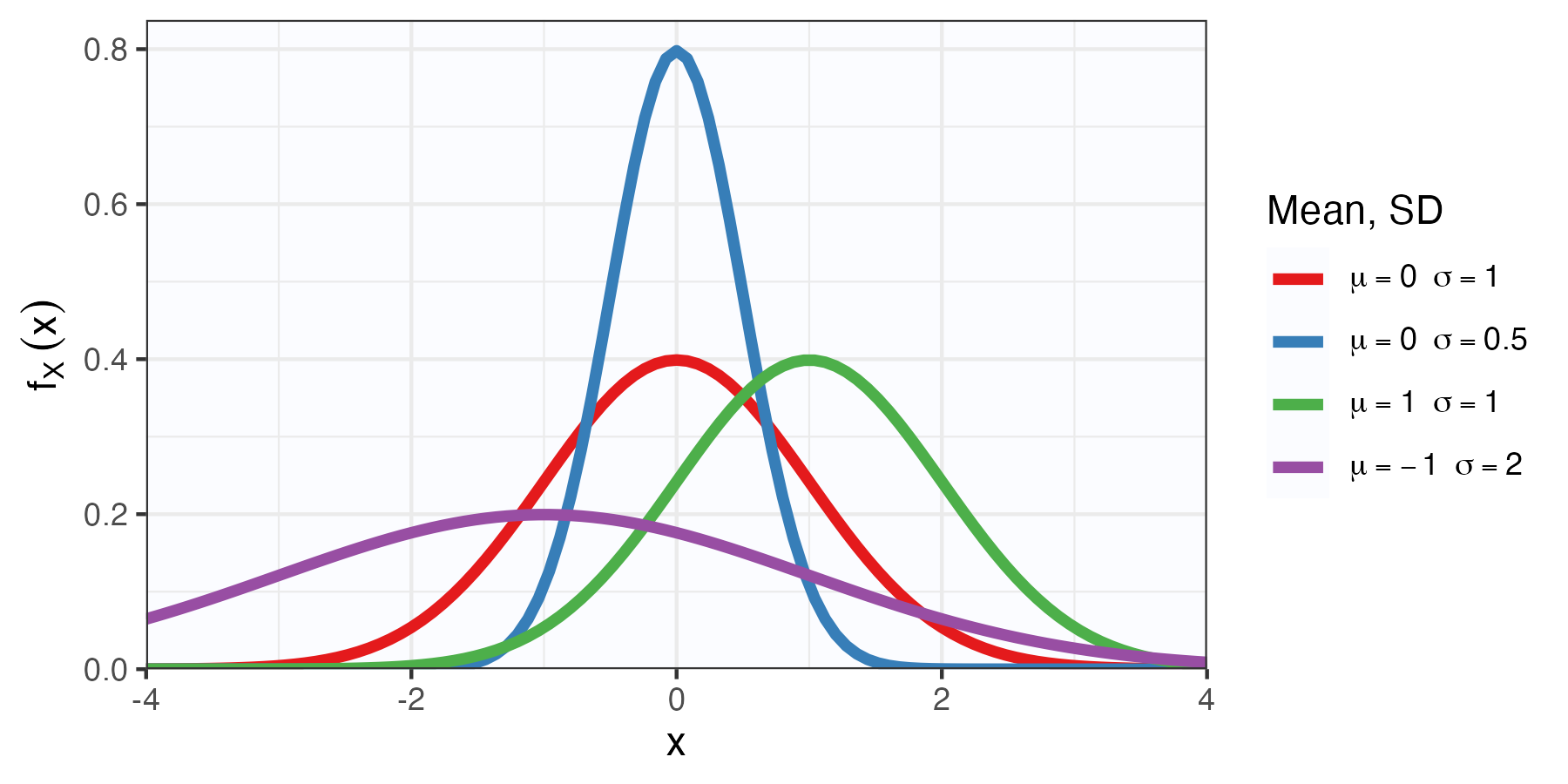
Let $\mu\in{\mathbb{R}}$, $\sigma>0$. A RV $Z$ with pdf \[f_Z(z; \mu, \sigma^2) = \frac{1}{\sqrt{2\pi\sigma^2}} \exp\left\{ -\frac{(z-\mu)^2}{2\sigma^2}\right\},\] is said to have the $\mathcal{N}(\mu, \sigma^2)$ distribution.

The Normal distribution, factoids

This distribution is incredibly important.
The reason is that it is good for modelling averages. We’ll justify this rigorously later.
$Z \sim \mathcal{N}(0,1)$ is called the standard normal distribution. When $Z$ is written without context, it is often understood to have this specific distribution.
Unfortunately \[\mathbb{P}(a<Z<b) = \int_a^b \frac{1}{\sqrt{2\pi}} e^{-z^2/ 2} \mathsf{d}z,\] does not have a closed form solution.
Old folks used tables in textbooks to calculate this (Table D.2 on p. 712 for you).
Nowadays, we use software.

2 Cumulative distribution functions (CDFs)

Cumulative distribution functions (CDFs)

Definition

The cumulative distribution function of a random variable $X$ is \[F_X(x) \, = \, \mathbb{P}\left( X \le x \right) \, , \qquad \mbox{ for } x \in {\mathbb{R}}\]

Theorem

Let $X$ be a random variable with CDF $F_X$. Then:

$0 \le F_X(x) \le 1$ for all $x \in {\mathbb{R}}$;
$F\left( x \right) \leq F(y)$ for all $x \leq y$;
$\lim_{a \to -\infty} F_X\left( a \right) =0$,
$\lim_{a \to +\infty} F_X\left( a \right) =1$

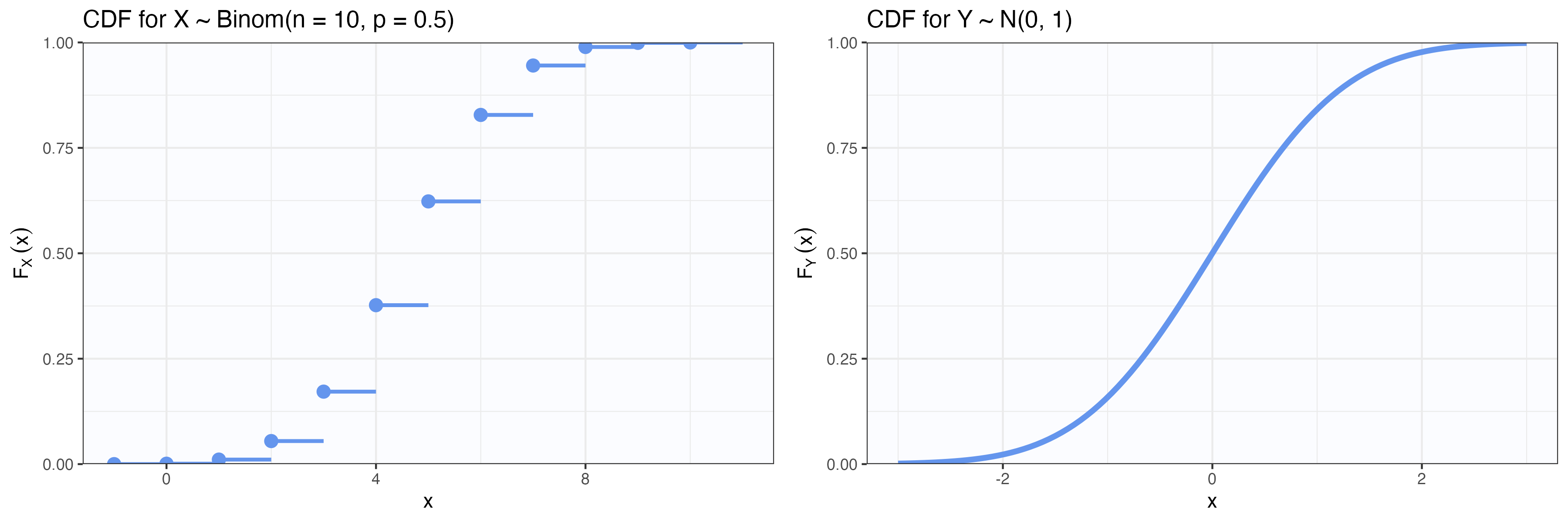
CDFs for discrete and continuous RVs

Discrete RV

\[F_X(x) = \sum_{t \leq x} p_X(t)\]

The CDF is a step function and right-continuous.

Continuous RV

\[F_X(x) = \int_{-\infty}^x f_X(t) \mathsf{d}t\]

The CDF is continuous (left and right limits are equal).

CDFs and distributions

Theorem

Let $X$ be any random variable with CDF $F_X$. Let $B$ be any subset of ${\mathbb{R}}$. Then $\mathbb{P}(X \in B)$ can be determined solely from $F_X$.

This is a very important result.
It means that the CDF contains all the information about the distribution of $X$.
It doesn’t matter whether $X$ is discrete, continuous, or anything else.
So the CDF “tells the whole story” about the distribution of $X$.

CDF of ${\mathrm{Exp}}(\lambda)$

Let $X \sim {\mathrm{Exp}}(\lambda)$, with pdf \[f_X(x) = \lambda e^{-\lambda x} I_{[0,\infty)}(x).\]

Exercise 2

Find $F_{X}\left(x \right)$.

Using CDFs to create new distributions

Proposition

Let $X_1, X_2,\dots$ be a random variables with CDFs $F_{X_1}, F_{X_2}, \dots$. Then the the following hold:

The RV $Y = X_1 + c$ has CDF $F_{X_1}(x - c)$;
The RV $Y = kX_1$ has CDF $F_{X_1}(x/k)$ for any $k > 0$;
For any constants $p_i$ such that $p_i \ge 0$ and $\sum_{i = 1}^k p_i = 1$, $F_G(x) = \sum_{i = 1}^k p_i F_{X_i}(x)$ is the CDF of the mixture of $F_{X_i}$.

There are various other similar results we could state.
One may mix discrete and continuous distributions using CDFs.

Mixture distributions

Consider the scores on Midterm 1 in a class. Suppose that there are three types of students, modelled as follows:

Poorly prepared students who did not study much (30%): $X_1 \sim \mathcal{N}(\mu = 50, \sigma = 10)$.
Well prepared students who studied a lot (60%): $X_2 \sim \mathcal{N}(\mu = 80, \sigma = 8)$.
Students who didn’t take the exam at all (10%): $X_3 = 0$ with probability 1.

Exercise 3

Find the CDF of the overall score distribution $X$. Write your answer in terms of the standard normal CDF $\Phi(\cdot)$.

Hint: If $Y \sim \mathcal{N}(\mu, \sigma)$, then $F_Y(y) = \Phi\left( \frac{y - \mu}{\sigma} \right)$.

3 Transformations of random variables

Transformations of a random variable

Let $X$ be a random variable with some distribution, and let $Y = g(X)$ for some function $g : {\mathbb{R}}\to {\mathbb{R}}$.

We want to find the distribution of $Y$.

The “Distribution method” just uses the definition:

\[\mathbb{P}(Y \in A) = \mathbb{P}(g(X) \in A) = \mathbb{P}(\{x : g(x) \in A\}).\]

If we can characterize these sets, we can find the distribution of $Y$. This method always works, and is easy for discrete random variables.

Theorem

Let $X$ be a discrete random variable with PMF $p_X(x)$. Let $Y = g(X)$ for some function $g : {\mathbb{R}}\to {\mathbb{R}}$. Then the PMF of $Y$ is given by \[p_Y(y) = \sum_{x : g(x) = y} p_X(x) = \sum_{x \in g^{-1}(y)} p_X(x).\]

Easy example of distribution method for discrete RVs

Let $X \sim {\mathrm{Binom}}(n, \theta)$, for some $\theta \in (0,1)$.
Let $Y = n - X$.

Find the PMF of $Y$.

We have that \[\begin{aligned} p_Y(y) &= \sum_{x : g(x) = y} p_X(x) = \sum_{x : n - x = y} p_X(x) \\ &= p_X(n - y) & \text{only one $x$ satisfies this}\\ &= \binom{n}{n - y} \theta^{n - y} (1 - \theta)^{y}I_{\{0,\dots,n\}}(n-y) & \text{definition of Binomial}\\ &= \binom{n}{y} (1 - \theta)^{y} \theta^{n - y}I_{\{0,\dots,n\}}(y) & \text{symmetry of binomial coeff.} \end{aligned}\]

Therefore, $Y \sim {\mathrm{Binom}}(n, 1 - \theta).$

Transformations of continuous random variables

For continuous random variables, you can also use the distribution method, and sometimes this is the easiest way.

The other common method is the “Jacobian method”

Theorem

Let $X$ be an (absolutely) continuous random variable, with density function $f_X$. Let $Y = h(X)$, where $h : {\mathbb{R}}\to {\mathbb{R}}$ is a function that is differentiable and monotonic. Then $Y$ is also absolutely continuous, and its density function $f_Y$ is given by \[f_Y(y) = f_X(h^{-1}(y)) \left| \frac{\mathsf{d}}{\mathsf{d}y} (h^{-1}(y)) \right|,\] where $h^{-1}(y)$ is the unique number $x$ such that $h(x) = y$.

Example using the Jacobian method

Let $X \sim {\mathrm{Unif}}(0,1)$.
Let $Y = -\log(X)$.

Find the PDF of $Y$.

Note that $h(x) = -\log(x)$ is monotonic on $(0,1)$, so we can use the Jacobian method. The support of $X$ is $(0,1)$, so $Y$ takes values in $(0, \infty)$.

We have that $h^{-1}(z) = e^{-z}$ and $\frac{\mathsf{d}}{\mathsf{d}z} h^{-1}(z) = -e^{-z}$.

\[\begin{aligned} f_Y(y) &= f_X(h^{-1}(y)) \left| \frac{\mathsf{d}}{\mathsf{d}y} (h^{-1}(y)) \right|\\ &= f_X(e^{-y}) \left| -e^{-y} \right| \\ &= 1 \times e^{-y} I_{(0, \infty)}(y). \end{aligned}\]

Therefore, $Y \sim {\mathrm{Exp}}(1)$.

Some transformations to practice

Exercise 4

Let $X \sim {\mathrm{Unif}}\left( -1,1\right)$. Use the distribution method to find the PDF of $Z = X^2$.
Let $X \sim {\mathrm{Gam}}(\alpha, \lambda)$. Use the Jacobian method to find the PDF of $Y = 1/X$.

4 Joint distributions

Joint distribution of several random variables

Suppose $X$ and $Y$ are two random variables.
We may be interested in their distributions separately.
But this ignores the relationship between $X$ and $Y$.

Definition

The joint CDF of the two random variables $X$ and $Y$ is defined by \[F_{X, Y} ( a, b ) = \mathbb{P}( X \le a, \, \ Y \le b).\]

Recall: \[\left\{ X \le a \, , \ Y \le b \right\} = \left\{ X \le a \right\} \cap \left\{ Y \le b \right\}.\]

Joint PMFs and PDFs

Let $X$ and $Y$ be two random variables with joint CDF $F_{X, Y}(x, y)$.

Definition

If $X$ and $Y$ are both discrete, then the joint PMF of $(X, Y)$ is defined by \[p_{X, Y} ( a, b ) = \mathbb{P}( X = a, \, Y = b).\]

Definition

The random variables $X$ and $Y$ are jointly (absolutely) continuous if there exists a density function $f_{X, Y}(x, y)$ such that for any set $A \subset \mathbb{R}^2$, we have \[\mathbb{P}\left( (X, Y) \in A \right) = \iint_A f_{X, Y}(x, y) \mathsf{d}x \mathsf{d}y.\]

Easy discrete example

Consider the experiment of rolling two fair dice.
Let $X$ be the lowest of the two rolls, $Y$ be the highest.

Find the joint PMF of $X$ and $Y$.

$f_{X,Y}(x, y)$	1	2	3	4	5	6
1	1/36	2/36	2/36	2/36	2/36	2/36
2	0	1/36	2/36	2/36	2/36	2/36
3	0	0	1/36	2/36	2/36	2/36
4	0	0	0	1/36	2/36	2/36
5	0	0	0	0	1/36	2/36
6	0	0	0	0	0	1/36

Marginal CDFs

Theorem

\[\begin{aligned} \lim_{a \to -\infty} F_{X, Y}(a, y) &= 0 & \forall y &\in {\mathbb{R}}.\\ \lim_{b \to -\infty} F_{X, Y}(x, b) &= 0 & \forall x &\in {\mathbb{R}}.\\ \lim_{a \to \infty, \ b \to \infty} F_{X, Y}(a, b) &= 1. \end{aligned}\]

Definition

The marginal CDFs of $X$ and $Y$ are defined by \[F_X(x) = \lim_{b \to \infty} F_{X, Y}(x, b), \qquad F_Y(y) = \lim_{a \to \infty} F_{X, Y}(a, y).\]

Marginal PMFs and PDFs

Theorem

If $X$ and $Y$ are discrete, then the marginal PMFs of $X$ and $Y$ are given by \[\begin{aligned} f_X(x) &= \sum_{y} f_{X, Y}(x, y), & \text{and}\quad f_Y(y) &= \sum_{x} f_{X, Y}(x, y). \end{aligned}\]

Theorem

If $X$ and $Y$ are continuous, then the marginal PDFs of $X$ and $Y$ are given by \[\begin{aligned} f_X(x) &= \int_{-\infty}^\infty f_{X, Y}(x, y) \mathsf{d}y, & \text{and}\quad f_Y(y) &= \int_{-\infty}^\infty f_{X, Y}(x, y) \mathsf{d}x. \end{aligned}\]

Important

All of this generalizes to more than two random variables.

Easy discrete example, continued

Consider the experiment of rolling two fair dice. Let $X$ be the lowest of the two rolls, $Y$ be the highest.

$f_{X,Y}(x, y)$	1	2	3	4	5	6
1	1/36	2/36	2/36	2/36	2/36	2/36
2	0	1/36	2/36	2/36	2/36	2/36
3	0	0	1/36	2/36	2/36	2/36
4	0	0	0	1/36	2/36	2/36
5	0	0	0	0	1/36	2/36
6	0	0	0	0	0	1/36

Exercise 5

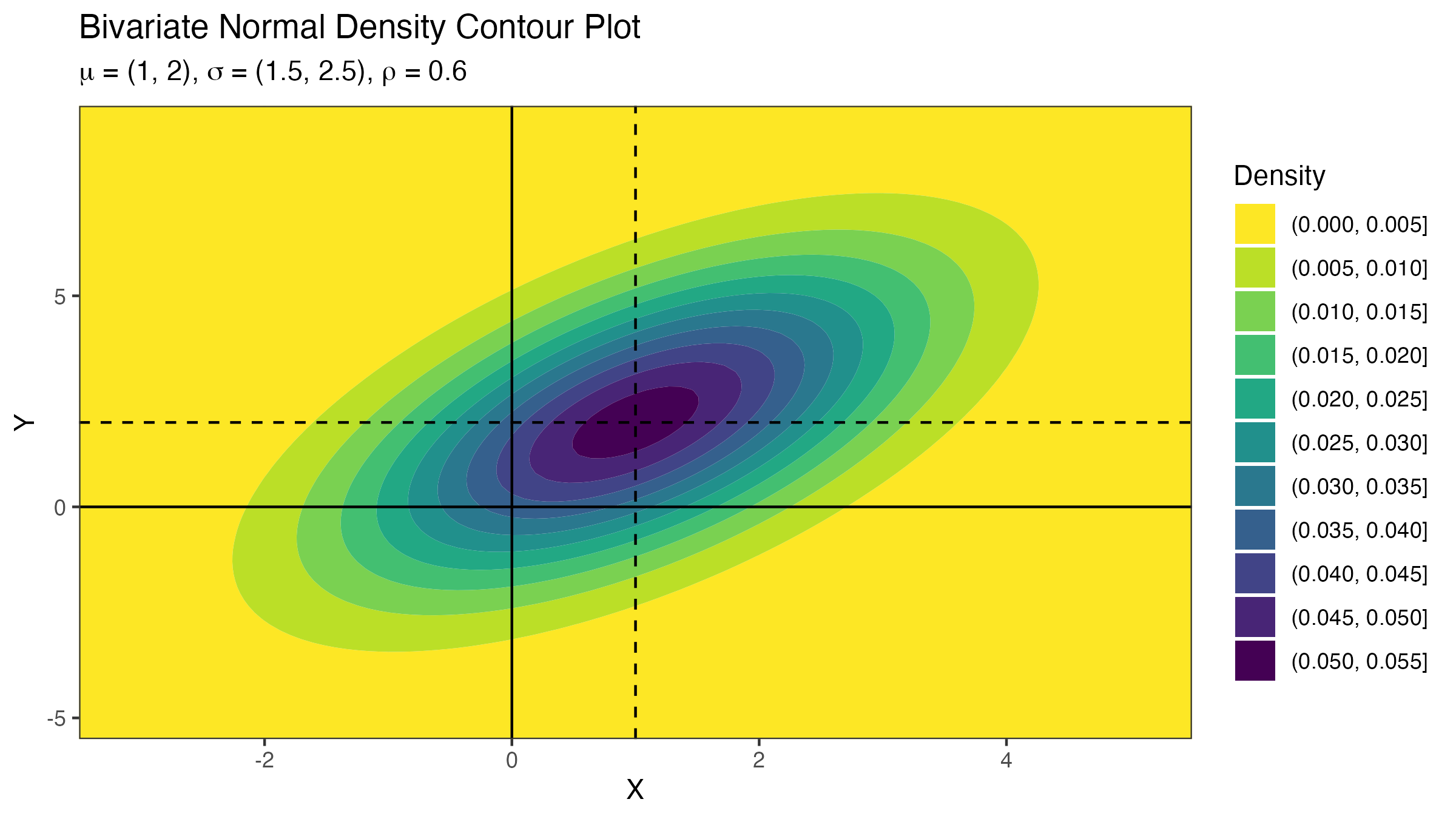
Find the marginal PMFs of $X$ and $Y$ from first principles, without using the joint PMF.
Use the joint PMF of $X$ and $Y$ to verify the marginal PMFs of $X$ and $Y$ are as found from first principles.

Multivariate Normal distribution

Definition

Given $\mu \in {\mathbb{R}}^p$ and a positive definite matrix $\Sigma \in {\mathbb{R}}^{p \times p}$, the multivariate normal distribution $\mathcal{N}(\mu, \Sigma)$, is the distribution of a random vector $X \in {\mathbb{R}}^p$ with density function \[f_X(x; \mu, \Sigma) = \frac{1}{(2\pi)^{p/2} |\Sigma|^{1/2}} \exp\left\{ -\frac{1}{2} (x - \mu)^{\mathsf{T}} \Sigma^{-1} (x - \mu) \right\},\] where $|\Sigma|$ is the determinant of $\Sigma$.

In the special case where $p=2$, $\mu = (\mu_1, \mu_2)^{\mathsf{T}}$, and $\Sigma = \begin{bmatrix} \sigma_1^2 & \rho \sigma_1 \sigma_2 \\ \rho \sigma_1 \sigma_2 & \sigma_2^2 \end{bmatrix}$, this “simplifies” to

\[\begin{aligned} &f_X(x; \mu, \Sigma)\\ &= \frac{1}{2\pi\sigma_1\sigma_2\sqrt{1 - \rho^2}} \exp\left\{ -\frac{1}{2(1 - \rho^2)} \left(\left(\frac{x_1-\mu_1}{\sigma_1}\right)^2 - 2\rho \frac{(x_1-\mu_1)(x_2-\mu_2)}{\sigma_1\sigma_2} + \left(\frac{x_2-\mu_2}{\sigma_2}\right)^2 \right) \right\}. \end{aligned}\]

Joint uniform distribution

Let $X$ and $Y$ be continuous random variables with PDF

\[ f_{X, Y}(x, y) = I_{[0,1]}(x)I_{[0,1]}(y) = I_{[0,1]^2}(x, y). \]

Exercise 6

Find $F ( x, y )$ for $0 \le x, y \le 1$;
Compute $F ( 0.3, 0.8 )$ and $F ( 0.3, 2.1 )$.
Calculate $P ( X - 2 Y > 0 )$.

Module 06

TC and DJM

1 Kernel matching and Gaussian distribution

Kernel and integration constant (review)

Kernel and integration constant: Example

Kernel matching

The Normal (Gaussian) distribution

The Normal distribution, factoids

2 Cumulative distribution functions (CDFs)

Cumulative distribution functions (CDFs)

CDFs for discrete and continuous RVs

CDFs and distributions

CDF of \({\mathrm{Exp}}(\lambda)\)

Using CDFs to create new distributions

Mixture distributions

3 Transformations of random variables

Transformations of a random variable

Easy example of distribution method for discrete RVs

Transformations of continuous random variables

Example using the Jacobian method

Some transformations to practice

4 Joint distributions

Joint distribution of several random variables

Joint PMFs and PDFs

Easy discrete example

Marginal CDFs

Marginal PMFs and PDFs

Easy discrete example, continued

Multivariate Normal distribution

Joint uniform distribution