Module 10
MGFs and conditional expectation
TC and DJM
Last modified — 21 Apr 2026
1 More on conditional expectation
Law of total expectation and variance (review)
Theorem
- The first equation shows what we just saw, but it is general and holds for any \(X\) and \(Y\).
- The second equation is a bit more complicated, but it is also very useful.
- It shows that the variance of \(X\) can be decomposed into two parts: the expected value of the conditional variance of \(X\) given \(Y\), and the variance of the conditional expectation of \(X\) given \(Y\).
Poisson/Gamma example
- Let \(\Lambda \sim {\mathrm{Gam}}(\alpha, \beta)\)
- Let \(X | \Lambda = \lambda \sim {\mathrm{Poiss}}(\lambda)\).
We want to find \(\mathbb{E}[X]\) and \(\operatorname{Var}(X)\).
- We have \[\mathbb{E}[X|\Lambda] = \Lambda \quad\text{and}\quad \operatorname{Var}(X|\Lambda) = \Lambda.\]
- Furthermore, \[\mathbb{E}[\Lambda] = \alpha / \beta \quad\text{and}\quad \operatorname{Var}(\Lambda) = \alpha / \beta^2.\]
Therefore \[\begin{aligned} \mathbb{E}[X] &= \mathbb{E}[\mathbb{E}[X|\Lambda]] = \mathbb{E}[\Lambda] = \alpha / \beta,\\ \operatorname{Var}(X) &= \mathbb{E}[\operatorname{Var}(X|\Lambda)] + \operatorname{Var}(\mathbb{E}[X|\Lambda]) = \mathbb{E}[\Lambda] + \operatorname{Var}(\Lambda) = \alpha / \beta + \alpha / \beta^2. \end{aligned}\]
Recognition
Exercise 1
Hint: There are two ways to do this. One solves ugly integrals, the other requires recognizing the distributions of \(X\) and \(Y|X\).
Cleaning up the properties of conditional expectation
- If \(X\) and \(Y\) are independent, then \[\mathbb{E}[ X | Y ] = \mathbb{E}[X],\quad\quad\text{and } \quad\quad\operatorname{Var}( X | Y ) = \operatorname{Var}(X).\]
- We can also calculate other conditional expectations, like the moment generating function.
Let \(X \sim {\mathrm{Poiss}}(\lambda)\) and \(Y | X = x \sim {\mathrm{Binom}}(x, \theta)\). Then,
\[\begin{aligned} m_Y(t) &= \mathbb{E}[ e^{t \, Y} ] = \mathbb{E}[ \, \mathbb{E}[ e^{t \, Y} | X ] ] = \mathbb{E}\left[ \left(\theta e^t + 1 - \theta \right)^X \right] =\sum_{x=0}^\infty \left(\theta e^t + 1 - \theta \right)^x \cdot \frac{\lambda^x e^{-\lambda}}{x!} \\ &= e^{-\lambda} \sum_{x=0}^\infty \frac{\left(\lambda \, \theta \, e^t + \lambda (1 - \theta)\right)^x}{x!} \quad\quad \text{kernel of ${\mathrm{Poiss}}(\lambda \, \theta \, e^t + \lambda (1 - \theta))$}\\ &= e^{-\lambda} \exp\left(\lambda \, \theta \, e^t + \lambda (1 - \theta)\right)\\ &= e^{\lambda \, \theta \left( e^t - 1 \right)} \quad\quad \text{MGF of ${\mathrm{Poiss}}(\lambda \, \theta)$}. \end{aligned}\]
Extra examples
Poisson MGF
Exercise
Hint: You should recall that the PMF of a Poisson random variable with parameter \(\lambda\) is \[p_X(x) = \frac{\lambda^x e^{-\lambda}}{x!}I_{\{0,1,2,\ldots\}}(x).\]
Using the Poisson MGF
Exercise
Sum of independent Poissons
Exercise
Discrete conditional expectation
Exercise
Let \(X\) and \(Y\) be two discrete random variables with joint PMF \[p_{X,Y}(x, y) = \frac{1}{11} I_{\{-4\}}(x) \bigg(I_{\{2\}}(y) + 2I_{\{3\}}(y) + 4I_{\{7\}}(y)\bigg) + \frac{1}{11} I_{\{6\}}(x) I_{\{2, 3, 7, 13\}}(y).\]
- Find \(p_X(x)\) and \(\mathbb{E}[X]\).
- Find \(\mathbb{E}[Y | X = -4]\) and \(\mathbb{E}[Y | X = 6]\).
- Find the distribution of \(\mathbb{E}[X | Y]\) as a function of \(Y\).
- Find \(\mathbb{E}[\mathbb{E}[X | Y]]\) and verify that it is equal to \(\mathbb{E}[X]\).
2 Inequalities
Markov’s Inequality
Theorem
Note that this implies that for any random variable \(Y\),
\[\mathbb{P}(|Y| \geq a) \le \mathbb{E}[|Y|] / a.\]
Proof of Markov’s Inequality
Proof
Chebyshev’s1 Inequality
Theorem
Then, for any \(a > 0\), \[\mathbb{P}(| X - \mu| \geq a ) \leq \ \frac{\operatorname{Var}(X)}{a^2}.\]
Proof
Comparing Markov and Chebyshev
Let \(X\) be a non-negative random variable with mean \(\mu\) and variance \(\mu\).
We want to examine the bounds on \(\mathbb{P}((X - \mu)/\mu \geq 1)\) given by Markov’s and Chebyshev’s inequalities.
Markov’s inequality gives \[\mathbb{P}((X - \mu)/\mu \geq 1) = \mathbb{P}( X \geq 2\mu ) \leq \ \frac{\mathbb{E}[X]}{2\mu} = \frac{\mu}{2\mu} = \frac{1}{2}.\]
Chebyshev’s inequality gives \[\mathbb{P}((X - \mu)/\mu \geq 1) = \mathbb{P}(X - \mu \geq \mu) \leq \mathbb{P}(|X - \mu| \geq \mu) \leq \frac{\operatorname{Var}(X)}{\mu^2} = \frac{\mu}{\mu^2} = \frac{1}{\mu}.\]
So for any random variable with mean \(\mu\) and variance \(\mu\), Chebyshev’s inequality gives a tighter bound whenever \(\mu > 2\).
Binomial bounds
Exercise 2
Far away stars
- Suppose that a radio telescope can measure the distance to a star.
- But due to atmospheric conditions, instrumental error, and movements of the earth, each measurement is a random variable with mean \(\mu\) light years (the true distance) and variance \(4\) (square) light years.
- An astronomer plans to take \(n\) independent measurements of the distance and use their average \(\overline{X}_n\) as an estimate for the true distance.
Exercise 3
Hint: recall that \(\mathbb{E}[ \overline{X}_n ] = \mathbb{E}[X_1]\) and \(\operatorname{Var}( \overline{X}_n ) = \operatorname{Var}(X_1)/n\).
Cauchy Schwarz Inequality
Theorem: Cauchy Schwarz for random variables
Corollary
If, in addition, \(\operatorname{Var}(X) > 0\) and \(\operatorname{Var}(Y) > 0\), then \[|\operatorname{Corr}(X, Y)| \leq 1.\]
Jensen’s Inequality
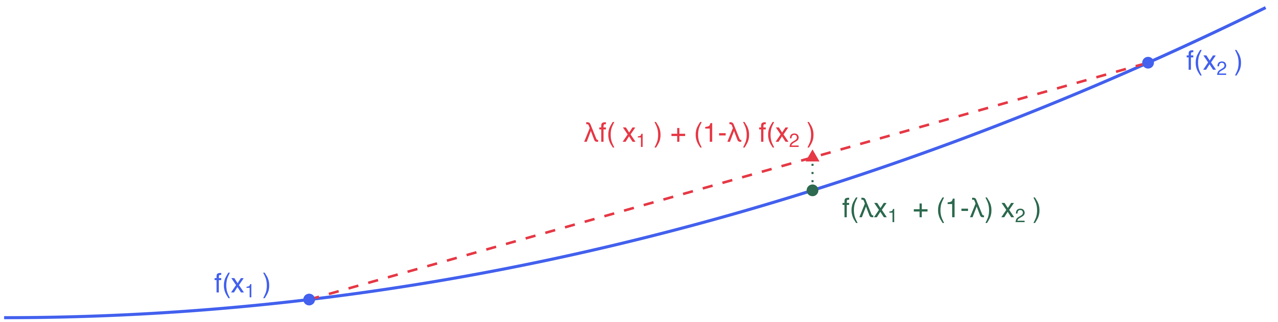
Recall that a function \(f: {\mathbb{R}}\to {\mathbb{R}}\) is convex if for any \(x, y \in {\mathbb{R}}\) and \(\lambda \in [0, 1]\), we have \[f(\lambda x + (1 - \lambda) y) \leq \lambda f(x) + (1 - \lambda) f(y).\]
Theorem
Questionable friendships
Exercise 4
- Your friend pays you $49 to roll 2 standard 6-sided dice.
- If you see \(x\) pips, you pay your friend $\(x^2\).
- Repeat as many times as you like, and your friend will keep paying you $49 each time.
How many times should you play this game? Justify your answer.
Followup on Jensen’s inequality
Exercise 5
Stat 302 - Winter 2025/26