Module 11

Convergence of random variables

TC and DJM

Last modified — 05 Apr 2026

1 Asymptotics

Convergence of numbers vs. convergence of random variables

In calculus, you looked at the limit of a sequence of numbers, $a_n$, as $n$ goes to infinity.

Example

$\lim_{n \to \infty} 1/n = 0;$
$\lim_{n \to \infty} (1 + 1/n)^n = e;$
$\lim_{n \to \infty} (1 + a/n)^n = e^a \text{ for all } a \in {\mathbb{R}};$
$\lim_{n \to \infty} (1 + a_n/n)^n = e^a \text{ if } a_n \to a.$

In probability, we look at the limit of a sequence of random variables, $X_n$, as $n$ goes to infinity.
This turns out to be more complicated, because there are different modes of convergence.

We will discuss 3 types of convergence.

Convergence in probability

Definition

A sequence of random variables $X_1,X_2,\ldots,X_n,\ldots$ converges in probability to a random variable $X$ if for all $\epsilon > 0$, \[\lim_{n \to \infty} \mathbb{P}(|X_n - X| < \epsilon) = 1.\]

We can think of $a_n = \mathbb{P}(|X_n - X| < \epsilon)$ as a sequence of numbers that goes to one as $n$ goes to infinity.
This is the most similar to limits of sequences of numbers.
Can also be written as $\mathbb{P}(|X_n - X| \geq \epsilon) \to 0$.
Common notation: $X_n \overset{p}{\to}X$.

Convergence in probability example

Let $U \sim {\mathrm{Unif}}(0,1)$ and define

\[X_n = U + B_n,\]

where $B_n\sim {\mathrm{Bern}}(1/n)$ are independent Bernoulli random variables, also independent of $U$.

Then $X_n\overset{p}{\to}U$.

\[\mathbb{P}(|X_n - U| > \epsilon) = \mathbb{P}\left(|B_n| > \epsilon\right) = \mathbb{P}(B_n = 1) = 1/n \to 0.\]

Convergence of maximum of i.i.d. Uniforms

Exercise 1

Let $U_1, U_2, \ldots$ be i.i.d. ${\mathrm{Unif}}(0,1)$ random variables. Define $Y_n = \max\{U_1, \ldots, U_n\}$.

Show that $Y_n \overset{p}{\to}1$.

Hint: $|Y_n - 1| > \epsilon$ if and only if $Y_n < 1 - \epsilon$.

Convergence almost surely (with probability one)

Definition

A sequence of random variables $X_1,X_2,\ldots,X_n,\ldots$ converges almost surely (or w.p. 1) to a random variable $X$ if for all $\epsilon > 0$, \[\mathbb{P}\left(\lim_{n \to \infty} |X_n - X| < \epsilon\right) = 1.\]

This is a stronger notion of convergence than convergence in probability.
This is equivalent to saying that $\mathbb{P}(\lim_{n \to \infty} X_n = X) = 1$.
Writing this statement more explicitly, we are really demanding that \[\mathbb{P}\left(\{\omega : \lim_{n \to \infty} X_n(\omega) = X(\omega)\}\right) = 1.\]
Common notation: $X_n \overset{a.s.}{\to}X$.

Same example, different convergence

Let $U \sim {\mathrm{Unif}}(0,1)$ and define

\[X_n = U + B_n\]

where $B_n\sim {\mathrm{Bern}}(1/n)$ are independent Bernoulli random variables, also independent of $U$.

Then $X_n$ does NOT converge almost surely to $U$. The proof is similar to Question 6 on the first exam.

\[\begin{aligned} \mathbb{P}(\{\omega : \lim_{n \to \infty} X_n(\omega) = U(\omega)\}) &= \mathbb{P}\left(\{\omega : \lim_{n \to \infty} B_n(\omega) = 0\}\right)\\ &= \mathbb{P}(\left\{\omega : \text{there exists } m \text{ such that, for all } n \geq m, B_n(\omega) = 0\right\})\\ &= \mathbb{P}\left(\bigcup_{m=1}^\infty \bigcap_{n=m}^\infty \{\omega: B_n(\omega) = 0\}\right) \\ &= \lim_{m \to \infty} \mathbb{P}\left(\bigcap_{n=m}^\infty \{B_n = 0\}\right)\\ &= \lim_{m \to \infty} \prod_{n=m}^\infty \mathbb{P}(B_n = 0) = \lim_{m \to \infty} \prod_{n=m}^\infty (1 - 1/n) = 0 \neq 1. \end{aligned}\]

Convergence in distribution

Definition

A sequence of random variables $X_1,X_2,\ldots,X_n,\ldots$ with CDFs $F_n$ converges in distribution to a random variable $X$ with CDF $F$ if, for all $t$ at which $F$ is continuous, \[\lim_{n \to \infty} F_n(t) = F(t).\]

We will see that this is the “weakest” notion of convergence.
But it gets used more frequently than the others.
Common notation: $X_n \overset{d}{\to}X$.

Proposition

If there exists $s>0$ such that for all $t \in (-s,s)$ $m_{X_n}(t) \to m_X(t)$, then $X_n \overset{d}{\to}X$.

Revisiting our convergence in probability example

Let $U \sim {\mathrm{Unif}}(0,1)$, and let $U_n\sim {\mathrm{Unif}}(0,1)$ all independent. Define

\[X_n = U_n + B_n\]

where $B_n\sim {\mathrm{Bern}}(1/n)$ are independent Bernoullis, also independent of $U, U_1, U_2, \ldots$.

Then $X_n\overset{d}{\to}U$ but $X_n$ does NOT converge in probability to $U$.

We have that, for all $t$, \[m_{X_n}(t) = m_{U_n}(t) m_{B_n}(t) = \frac{e^t - 1}{t} (1-\frac{1}{n} + \frac{1}{n}e^t) \to \frac{e^t - 1}{t} = m_U(t).\]

However, \[\begin{aligned} \mathbb{P}(|X_n - U| > \epsilon) &= \mathbb{P}\left(|U_n + B_n - U| > \epsilon\right) \\ &= (1-1/n)\mathbb{P}\left(|U_n - U| > \epsilon\right) + (1/n)\mathbb{P}\left(|U_n +1- U| > \epsilon\right) \\ &= (1-1/n)(1-\epsilon)^2 + (1/n)a \quad\quad\text{for some $a\in[0,1]$}\\ &\rightarrow (1-\epsilon)^2 \neq 0. \end{aligned}\]

Normal MGF convergence

Exercise 2

Let $X_n\sim \mathcal{N}(0, 1 + 1/n)$ for all $n$, mutually independent. Show that $X_n \overset{d}{\to}Z\sim\mathcal{N}(0,1)$ by examining the moment generating functions.

Hint: Recall that the MGF of $\mathcal{N}(\mu, \sigma^2)$ is $m(t) = e^{\mu t + \sigma^2 t^2/2}$.

Relationships between different types of convergence

Theorem

The following implications hold for any sequence of random variables $X_1, X_2, \ldots$ and any random variable $X$: \[ X_n \overset{a.s.}{\to}X \Longrightarrow X_n \overset{p}{\to}X \Longrightarrow X_n \overset{d}{\to}X. \]

Interpreting convergence

Convergence almost surely (with probability 1) is examining the sample path of $X_n(\omega)$. We need this path to converge to the value of $X(\omega)$ for almost all $\omega$.
Convergence in probability involves the joint distribution of $X_n$ and $X$: we are looking at the probability that $|X_n - X|$ is small. We hope this probability goes to one.
Convergence in distribution only involves the marginal distribution of $X_n$. We are looking at the distribution of $X_n$ and hoping it gets closer and closer to the distribution of $X$ as $n$ increases.

Visualization of convergence

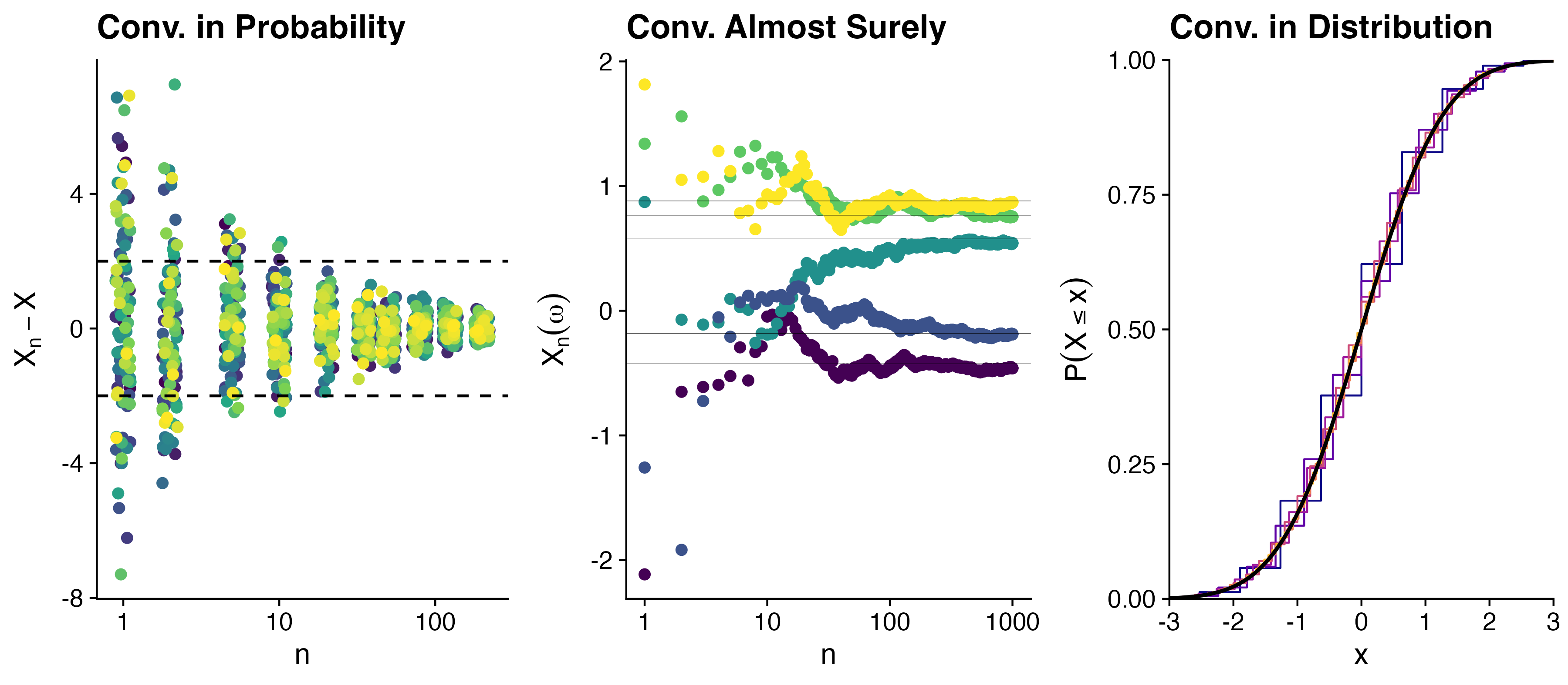
The probability that $X_n - X$ is large shrinks as $n$ increases. (100 samples from $X_n - X$)
For each $\omega$, the sample path $X_n(\omega)$ gets closer and closer to $X(\omega)$ as $n$ increases.
The CDF of $X_n$ gets closer and closer to the CDF of $X$ as $n$ increases.

Convergence of maximum of i.i.d. Uniforms

Exercise 3

Let $U_1, U_2, \ldots$ be i.i.d. ${\mathrm{Unif}}(0,1)$ random variables. Define $Y_n = \max\{U_1, \ldots, U_n\}$.

Show that $n(1-Y_n) \overset{d}{\to}{\mathrm{Exp}}(1)$.

Hints:

Start by finding the CDF $F_{Y_n}(t)$ of $n(1-Y_n)$.
Recall that the CDF of ${\mathrm{Exp}}(1)$ is $F(t) = 1 - e^{-t}$.

Normal convergence, continued

Exercise 4

Let $X_n\sim \mathcal{N}(0, 1 + 1/n)$, mutually independent, for all $n$. Does $X_n \overset{p}{\to}Z\sim\mathcal{N}(0,1)$? Justify your answer.

2 Convergence of means (and sums)

Weak Law of Large Numbers (WLLN)

Theorem

Let $X_{1},X_{2}, \ldots, X_{n} \, \ldots$ be independent and identically distributed (i.i.d) random variables with finite mean $\mu$. Then,

\[\overline{X}_n = \frac{1}{n} \, \sum_{i=1}^n X_i \overset{p}{\to}\mu.\]

Interpretation

The distribution of $\overline{X}_n$ gets more and more concentrated around $\mu$ as $n$ increases.

So many dice

Exercise 5

Let $X_n$ be the sum of the squares of $n$ independent rolls of a fair six-sided die.

That is \[X_n = \sum_{i=1}^n X_{n,i}^2,\] where $X_{n,i}$ is the result of the $i$-th die roll.

Show that $n^{-1}X_n \overset{p}{\to}m$ for some $m$ (find $m$ explicitly).

Proof of WLLN with an extra condition

Proof

Assume that $\operatorname{Var}( X_{i}) =\sigma ^{2} < \infty$ (same for all $i$). This is not required for the WLLN, but it makes the proof easier.

Then, by Chebyshev’s inequality, for all $\epsilon > 0$, \[\begin{aligned} \mathbb{P}\left( \left\vert \overline{X}_n-\mu \right\vert \geq \epsilon \right) &\leq \frac{\operatorname{Var}(\overline{X}_n)}{\epsilon^2} = \frac{\sigma^2/n}{\epsilon^2} \to 0. \end{aligned}\]

The Central Limit Theorem (CLT)

Theorem

Let $X_{1},X_{2}, \dots, X_n,\ldots$ be i.i.d random variables with finite mean $\mu$ and variance $\sigma^2$.

Then, \[ \frac{\sqrt{n}(\overline{X}_n-\mu )}{\sigma } \overset{d}{\to}\mathcal{N}\left( 0,1\right). \]

People often say that $\overline{X}_n$ converges to a standard Gaussian.
They mean that $\overline{X}_n$ appropriately normalized converges.

Interpretation

Probability statements about $\overline{X}_n$ can be approximated using a Normal distribution. It’s the probability statements that we are approximating, not the random variable itself.

Importance of normalization

Warning

What happens if we don’t normalize?

The WLLN tells us that $\overline{X}_n \overset{p}{\to}\mu$.
Defining $Y_n = (X_n - \mu)/\sigma$, we have $\overline{Y}_n = (\overline{X}_n - \mu)/\sigma$.
But, we also know that $\mathbb{E}[Y_n] = 0$ and $\operatorname{Var}(Y_n) = 1$ for all $n$.
So the LLN tells us that $\overline{Y}_n \overset{p}{\to}0$.

Interpretation

Multiplying by $\sqrt{n}$ prevents the distribution of $\overline{Y}_n$ from collapsing to a point mass at $0$ as $n$ increases, and allows us to get a non-degenerate limit distribution.

Equivalent statements of the CLT

Define \[Z_n = \frac{\sqrt{n}(\overline{X}_n-\mu )}{\sigma }.\]

There are several forms of notation that all basically say the same thing. \[\begin{aligned} Z_n &\approx \mathcal{N}(0,1)\\ \overline{X}_n &\approx \mathcal{N}\left(\mu, \frac{\sigma^2}{n}\right)\\ \overline{X}_n - \mu &\approx \mathcal{N}\left(0, \frac{\sigma^2}{n}\right)\\ \sqrt{n}(\overline{X}_n - \mu) &\approx \mathcal{N}(0, \sigma^2)\\ \frac{\overline{X}_n - \mu}{\sigma/\sqrt{n}} &\approx \mathcal{N}(0,1). \end{aligned}\]

Things you should not say

You should not say things like:

\[\overline{X}_n \overset{d}{\to}\mathcal{N}(\mu, \sigma^2/n).\]

This creeps me out because you are taking a limit on the left-hand side where $n$ goes to infinity, but the distribution on the right-hand side still depends on $n$.

Usefulness of the CLT

In many situations, the exact distribution of $\overline{X}_n$, $\mathbb{P}(\overline X_n \leq x)$, is hard to determine exactly.
The CLT allows us to approximate this value by

\[\mathbb{P}(\overline X_n \leq x) \approx \Phi\Big ( \frac{\sqrt{n}(x-\mu)}{\sigma}\Big )\] with a respectable precision when $n$ is large.

Some people say that this approximation has acceptable precision when $n \ge 30$.
Ignore those people.
It would be more accurate to say “if $n<30$, this approximation is probably bad”.

Far away stars, revisited

Suppose that a radio telescope can measure the distance to a star.
But due to atmospheric conditions, instrumental error, and movements of the earth, each measurement is a random variable with mean $\mu$ light years (the true distance) and variance $4$ (square) light years.
An astronomer plans to take $n$ independent measurements of the distance and use their average $\overline{X}_n$ as an estimate for the true distance.

Exercise 6

Use the CLT to determine how many measurements the astronomer should make if they want the probability of a mismeasurement larger than 1 light year to be no more than 0.01?

Far away stars, Discussion

Chebyshev’s inequality suggests \[n \ge 400\] independent observations.
CLT suggests \[n \ge 27\] independent observations
Both are correct, but the CLT is more precise.
To be fair, it used more information (the asymptotic distribution of the sample mean), which may or may not be accurate.
Chebyshev’s doesn’t use any approximation, it’s a guarantee.

Proof of the CLT

Let $Z_n = \frac{\sqrt{n}(\overline{X}_n-\mu )}{\sigma}$ as before.

Define $Y_i = (X_i - \mu)/\sigma$ for all $i$.

Then, $Y_1, Y_2, \ldots$ are i.i.d. with mean $0$ and variance $1$, and we have $\frac{1}{\sqrt{n}}\sum_{i=1}^n Y_i = Z_n.$

By the proposition about MGFs, we need to show that $m_{Z_n}(t) \to m_Z(t)$ for all $t,$ where $Z\sim \mathcal{N}(0,1)$.

Suppose that $Y_i$ has moment generating function $m_Y(t)$.

Then, the moment generating function of $\sum Y_i$ is $m_Y(t)^n$.

Therefore, the moment generating function of $Z_n$ is $m_Y(t/\sqrt{n})^n$.

Proof of the CLT, continued

Now, $m'_Y(0) = \mathbb{E}[Y_i] = 0$ and $m''_Y(0) = \mathbb{E}[Y_i^2] = 1$.

By Taylor’s theorem, for all $t$, \[\begin{aligned} m_Y(t) &= m_Y(0) + m'_Y(0)t + \frac{1}{2}m''_Y(0)t^2 + \cdots\\ &= 1 + 0 + \frac{t^2}{2} + \frac{t^3}{3!}m'''_Y(0) + \cdots \\ &= 1 + \frac{t^2}{2} + \frac{t^3}{3!}m'''_Y(0)+ \cdots.\\ \Longrightarrow \quad m_{Z_n}(t) &= m_Y(t/\sqrt{n})^n \ = \left(1 + \frac{\frac{t^2}{2} + \frac{t^3}{3!n^{1/2}}m'''_Y(0) + \cdots}{n}\right)^n \to e^{t^2/2} = m_Z(t). \end{aligned}\]

[We used the fact that $\lim_{n \to \infty} (1 + a_n/n)^n = e^a$ when $a_n \to a$.]

Central Limit Theorem for i.i.d. sums

The CLT states that when $n$ is large, the distribution of \[\frac{\overline{X}_n - \mu }{\sigma /\sqrt{n}} \text{ \ \ is \ approximately \ } \mathcal{N}\left( 0,1\right).\]
This implies that when $n$ is large, we can also say something about the distribution of $S_n = \sum_{i=1}^{n}X_{i}$.

\[\begin{aligned} 1-\Phi(z) &= \lim_{n\rightarrow\infty}\mathbb{P}\left( \frac{\overline X_n - \mu} {\sigma/\sqrt{n}} > z \right)\\ &=\lim_{n\rightarrow\infty}\mathbb{P}\left( \frac{(n\overline X_n - n\mu)} {n\sigma/\sqrt{n}} > z \right)\\ &=\lim_{n\rightarrow\infty}\mathbb{P}\left( \frac{S_n - n\mu} {\sqrt{n}\sigma} > z \right) \end{aligned}\]

Struggling restaurants

The daily sales on any given day of a restaurant is a random variable with mean $2500 and SD $500.
Assume that daily sales are independent random variables.

Exercise 7

Give an approximate value of the probability that the total sale for the 30 days will be over $80,000.

Leave your answer in terms of $\Phi$ (the CDF of a standard Gaussian).

What was the point of all this?

Why probability theory?

Probability theory is the mathematical framework for modeling and analyzing random phenomena.
We started by examining simple experiments (like gambling) where we had a good understanding of the underlying probability model.
Then we abstracted away from the sample space and focused on the properties of random variables, which are functions of the outcomes of the experiment.
We have developed tools to analyze the behavior of random variables, such as expectation, variance, and conditional expectation.
All of these tools are useful for understanding randomness at particular levels of granularity.

Why probability theory?

The more precise we can be about the distribution of a random variable, the more precise our conclusions can be.
But with more precision comes more assumptions about how the world works, and more assumptions means more risk of being wrong.
Inequalities like Markov’s and Chebyshev’s allow us to understand the behavior of random variables without needing to know their exact distribution.
Asymptotic results allow us to approximate possibly unknown distributions with things we understand better.

Why probability theory?

The field of Statistics turns the operation around.

We collected data, which we can think of as realizations of random variables.
If we make (some) assumptions about the random process that generated the data, then we can understand the underlying probability model (and future data from that model).
Usually we only know parts of the process, but not all the details (parameters, etc.).
This is the basis of statistical inference — the process of using data to learn about the underlying random variable and the processes that generate it.

Summary

Stat302 gives (gave?) you the tools to understand the behavior of random variables — the foundation for understanding statistical inference.