Module 3

Matias Salibian Barrera

Last modified — 29 Sep 2025

Conditional probability

• In general, the outcome of a random experiment can be any element of \(\Omega\).

• Sometimes, we have “partial information” about the outcome.

• Example: Roll a dice. If \(A\) is the even of obtaining a “2”, then \(\mathbb{P}(A) = 1/6\).

• But if the outcome is known to be even, then the chance should be higher.

Conditional probability

• These two events play distinct roles in this example:

  • The event of interest \(A\):  \(A = \{ 2 \}\)

  • The conditioning event \(B\), the “partial information”: \[B = \{ 2, 4, 6 \}\]

Conditional probability

• Let \(A, B \subseteq \Omega\) and assume \(\mathbb{P}(B) > 0\)

• The conditional probability of \(A\) given \(B\) is \[\mathbb{P}\left(A \ \vert\ B \right) \, = \, \frac{ \mathbb{P}\left( A \cap B \right) }{ \mathbb{P}\left( B \right) }\]

• For any fixed \(B\), the function \[\mathbb{Q}_B \left( \ \cdot \ \right) \, = \, \mathbb{P}\left(\ \cdot \ \ \vert\ B \right)\] satisfies the three Axioms of a Probability.

The dot in “\(\mathbb{Q}_B(\cdot)\)” is meant to highlight the fact that \(\mathbb{Q}_B\) is a function, its argument is any event \(A \subseteq \Omega\).

Proof that \(Q\) is a probability

• Axiom 1: \(\mathbb{Q}_B \left( \Omega \right) = 1\):
  • Proof: \[\mathbb{Q}_B \left( \Omega \right) = \frac{ \mathbb{P}\left( \Omega \cap B \right) }{\mathbb{P}\left( B \right) } = \frac{ \mathbb{P}\left( B \right) }{ \mathbb{P}\left( B \right) } = 1\]
• Axiom 2: \(\mathbb{Q}_B \left( A \right) \ge 0\) for any \(A \in \Omega\):
  • Proof: \[\mathbb{Q}_B \left( A \right) = \frac{ \mathbb{P}\left( A \cap B \right) }{\mathbb{P}\left( B \right) } \ge 0\]

Proof that \(Q\) is a probability (cont’d)

• Axiom 3: If \(\left\{ A_i \right\}_{i \ge 1}\) are disjoint events:
  • Proof: \[\begin{aligned} \mathbb{Q}_B \left( \bigcup_{i=1}^\infty A_i \right) & = \ \bigl. \mathbb{P}\biggl( \Bigl[ \bigcup_{i=1}^\infty A_i \Bigr] \bigcap B \biggr) \bigr/ \mathbb{P}\left( B \right) \\ & = \bigl. \mathbb{P}\Bigl( \bigcup_{i=1}^\infty \left[ A_i \cap B \right] \Bigr) \bigr/ \mathbb{P}\left( B \right) \\ & = \bigl. \left[ \sum_{i=1}^\infty \mathbb{P}\left( A_i \cap B \right) \right] \bigr/ \mathbb{P}\left( B \right) \\ & = \sum_{i=1}^\infty \frac{ \mathbb{P}\left( A_i \cap B \right) }{ \mathbb{P}\left( B \right) } \\ & = \sum_{i=1}^\infty \mathbb{Q}_B \left( A_i \right)\end{aligned}\]

Example of conditional probability

We roll a fair die, once, and record the outcome.

Consider the following events:

• \(A=\left\{ \text{4 or higher}\right\} =\{4,5,6\}\),

• \(B=\left\{ \text{even number}\right\} =\{2,4,6\}\)

• \(A\cap B=\left\{ 4,6\right\}\)

• Therefore \[\mathbb{P}\left( A\ \vert\ B\right) =\frac{\mathbb{P}\left( A\cap B\right) }{\mathbb{P}\left( B\right) }=\frac{% 1/3}{1/2}=2/3\]

Conditional probability

• \(\mathbb{P}\left( A\right) =0.50\),

• Knowing that the outcome is even increases this probability to \[\mathbb{P}\left( A\ \vert\ B\right) =0.667\]

• Alternatively, if we knew that \[C=\left\{ \text{the number is odd}\right\}\] then we would have: \[\mathbb{P}\left( A\ \vert\ C\right) =\frac{\mathbb{P}\left( A\cap C\right)}{\mathbb{P}\left( C\right) }=\frac{% 1/6}{1/2}=0.333\]

Multiplication property

• Notation: \(\mathbb{P}\left( A\ \vert\ B\right) =\) “probability of \(A\) given \(B\)”

• If \(\mathbb{P}(A_1) > 0\), then, \[\mathbb{P}\left( A_{1}\cap A_{2}\right) = \mathbb{P}\left( A_{2}\ \vert\ A_{1}\right) \, \mathbb{P}\left( A_{1}\right)\]

• More in general: \[\begin{aligned} \mathbb{P}\left( A_{1}\cap A_{2}\cap \cdots \cap A_{n}\right) \, &= \, \mathbb{P}\left( A_{n}\ \vert\ A_{1}\cap A_{2}\cap \cdots \cap A_{n-1}\right) \ \times \\ & \\ & \quad \times \ \mathbb{P}\left( A_{n-1}\ \vert\ A_{1}\cap A_{2}\cap \cdots \cap A_{n-2}\right) \ \times \\ & \\ & \quad \times \cdots \times \ \mathbb{P}\left( A_{3}\ \vert\ A_{1}\cap A_{2}\right) \times \mathbb{P}\left( A_{2}\ \vert\ A_{1}\right) \ \times \ \mathbb{P}\left( A_{1}\right) \end{aligned}\]

Conditional probability

Proof: To fix ideas, look at the case \(n=4\) \[\begin{aligned} \mathbb{P}\left( A_{1}\right) \, \mathbb{P}\left( A_{2}\ \vert\ A_{1}\right) \, \mathbb{P}\left( A_{3}\ \vert\ A_{1}\cap A_{2}\right) \, \mathbb{P}\left( A_{4}\ \vert\ A_{1}\cap A_{2}\cap A_{3}\right) &= \\ &&\end{aligned}\] \[\begin{aligned} &= \mathbb{P}\left( A_{1}\right) \, \frac{\mathbb{P}\left( A_{1}\cap A_{2}\right) }{\mathbb{P}\left( A_{1}\right) } \, \frac{\mathbb{P}\left( A_{1}\cap A_{2}\cap A_{3}\right) }{\mathbb{P}\left( A_{1}\cap A_{2}\right) } \, \frac{\mathbb{P}\left( A_{1}\cap A_{2}\cap A_{3}\cap A_{4}\right) }{\mathbb{P}\left( A_{1}\cap A_{2}\cap A_{3}\right) }= \\ &&\end{aligned}\] \[=\mathbb{P}\left( A_{1}\cap A_{2}\cap A_{3}\cap A_{4}\right)\] The general proof is the same, but requires more space

Conditional probability. An example

• An urn has 10 red balls and 40 black balls.

• Three balls are randomly drawn without replacement. Calculate the probability that:

  1. The first drawn ball is red, the 2nd is black and the 3rd is red.

  2. The 3rd ball is red given that the 1st is red and the 2nd is black.

Solution to (a)

• Event of interest: first is red, second is black and third is red

• Let \[R_{i} \, = \, \left\{ \mbox{the } i^{th} \mbox{ ball is red } \right\}\] \[B_{j} \, = \, \left\{ \text{ the } j^{th} \mbox{ ball is black }\right\}\]

• The event of interest is \[R_{1}\cap B_{2}\cap R_{3}\]

Answer by using multiplication rule

• We have \[\begin{aligned} \mathbb{P}\left( R_{1}\cap B_{2}\cap R_{3}\right) &= \mathbb{P}\left( R_{3}\ \vert\ R_{1}\cap B_{2}\right) \, \mathbb{P}\left( B_{2}\ \vert\ R_{1}\right) \, \mathbb{P}\left( R_{1}\right) \\ && \\ &=\frac{9}{48} \times \frac{40}{49}\times \frac{10}{50} = 0.031.\end{aligned}\]

Example, part (b)

• third ball is red given that the first is red and the second is black

• Event of interest: \(R_{3}\)

• Conditioning event: \(R_{1}\cap B_{2}\). We want \[\mathbb{P}\left( R_{3}\ \vert\ R_{1}\cap B_{2}\right) =\frac{\mathbb{P}\left( R_{1}\cap B_{2}\cap R_{3}\right) }{\mathbb{P}\left( R_{1}\cap B_{2}\right) }\]

• Using part (a) we have \[\mathbb{P}\left( R_{1}\cap B_{2}\cap R_{3}\right) = 0.031\]

Example, part (b)

• Also \[\mathbb{P}\left( R_{1}\cap B_{2}\right) = \mathbb{P}\left( B_{2}\ \vert\ R_{1}\right) \, \mathbb{P}\left( R_{1}\right) = \frac{40}{49} \times \frac{10}{50} = 0.16327\]

• Finally: \[\mathbb{P}\left( R_{3}\ \vert\ R_{1}\cap B_{2}\right) =\frac{0.031}{0.16327} = 0.18987\]

Total probability formula

• We say that \(B_{1}, \ldots, B_{n}\) is a partition of \(\Omega\) if

  • They are disjoint \[B_{i}\cap B_{j} \, = \, \varnothing \quad \mbox{ for } i \ne j \, ,\]

  • They cover the whole sample space: \[\bigcup_{i=1}^{n} B_{i} \, = \, \Omega\]

• In that case, for any \(A \in \Omega\): \[\mathbb{P}\left( A\right) =\sum_{i=1}^{n} \mathbb{P}\left( A\ \vert\ B_{i}\right) \, \mathbb{P}\left( B_{i}\right)\]

Total probability formula: proof

• To prove it, note

  • \(A = A \cap \Omega =A \cap \left( \bigcup _{i=1}^{n}B_{i}\right) = \bigcup _{i=1}^{n}\left( A \cap B_{i}\right)\)

  • The events \(\left( A \cap B_{i}\right)\) are disjoint.

• Therefore, using Axiom 3, we have \[\begin{aligned} \mathbb{P}\left( A\right) & = \mathbb{P}\left( \bigcup_{i=1}^{n} A \cap B_{i} \right) \\ & \\ &=\sum_{i=1}^{n} \mathbb{P}\left( A\cap B_{i}\right) \\ && \\ &=\sum_{i=1}^{n} \mathbb{P}\left( A\ \vert\ B_{i}\right) \, \mathbb{P}\left( B_{i}\right) \end{aligned}\]

Spam email example

• Suppose that 1% of all email traffic is spam

• Assume that 90% of all spam email IS WRITTEN IN ALL CAPS

• Suppose that only 2% of not spam email is written in all caps

• If you receive an email, what is the probability that it is ALL IN CAPS?

Spam email example

• Let \[\begin{aligned} S &= \left\{ \mbox{ email is spam } \right\} &C &= \left\{ \mbox{ email IS ALL IN CAPS } \right) \end{aligned}\]

• We need to find \(P \left( C \right)\).

• \(S\) and \(S^c\) are a partition of \(\Omega\)

• Also, we know \[\mathbb{P}\left( S \right) = 0.01 \, , \quad \mathbb{P}\left( C \ \vert\ S \right) = 0.90 \, , \quad \mathbb{P}\left( C \ \vert\ S^c \right) = 0.02\]

• Then \[\begin{aligned} \mathbb{P}\left( C \right) & = \mathbb{P}\left( C \ \vert\ S \right) \, \mathbb{P}\left( S \right) + \mathbb{P}\left( C \ \vert\ S^c \right) \, \mathbb{P}\left( S^c \right) \\ & \\ & = 0.90 \times 0.01 + 0.02 \times 0.99 \\ & \\ & = 0.0288 \end{aligned}\]

Bayes formula

• Suppose \(B_{1}\), \(B_{2}\), …, \(B_{n}\) is a partition of the sample space

• Then, for each \(i=1,...,n\) we have: \[\mathbb{P}\left( B_{i}\ \vert\ A\right) \, = \, \frac{\mathbb{P}\left( A\ \vert\ B_{i}\right) \, \mathbb{P}\left( B_{i}\right) }{% \sum_{j=1}^{n} \mathbb{P}\left( A\ \vert\ B_{j}\right) \, \mathbb{P}\left( B_{j}\right) }\]

Bayes formula

• The proof is very simple: \[\begin{aligned} \mathbb{P}\left( B_{i}\ \vert\ A\right) &=\frac{\mathbb{P}\left( A\cap B_{i}\right)}{\mathbb{P}\left( A\right) } & \text{(Definition of conditional prob)} \\ &=\frac{ \mathbb{P}\left( A\ \vert\ B_{i}\right) \, \mathbb{P}\left( B_{i}\right)}{\mathbb{P}\left( A\right) } & \text{(Multiplication Rule)} \\ &=\frac{\mathbb{P}\left( A\ \vert\ B_{i}\right) \, \mathbb{P}\left( B_{i}\right) }{\sum_{j=1}^{n} \mathbb{P}\left( A\ \vert\ B_{j}\right) \, \mathbb{P}\left( B_{j}\right) } & \text{(Rule of Total Prob)} \end{aligned} \]

Spam email example

• Suppose that 1% of all email traffic is spam

• Assume that 90% of all spam email IS WRITTEN IN ALL CAPS

• Suppose that only 2% of not spam email is written in all caps

• If you receive an email what is the probability that it is spam? \[\mathbb{P}\left( \mbox{ email is spam } \right) = 0.01\]

• If the email IS ALL IN CAPS, what is the probability that it is spam? \[\mathbb{P}\left( \mbox{ email is spam } \ \vert\ \mbox{ IS ALL IN CAPS } \right) = \, ?\]

Spam email example

• Let \[S = \left\{ \mbox{ email is spam } \right\} \quad \quad C = \left\{ \mbox{ email IS ALL IN CAPS } \right)\]

• We need to find \(\mathbb{P}\left( S \ \vert\ C \right)\).

• We know \[\mathbb{P}\left(S \right) = 0.01 \, , \quad \mathbb{P}\left( C \ \vert\ S \right) = 0.90 \, , \text{ and } \quad \mathbb{P}\left( C \ \vert\ S^c \right) = 0.02\]

• Then \[\begin{aligned} \mathbb{P}\left( S \ \vert\ C \right) &= \frac{\mathbb{P}\left( C \ \vert\ S \right) \, \mathbb{P}\left( S \right)}{\mathbb{P}\left( C \right) } = \frac{\mathbb{P}\left( C \ \vert\ S \right) \, \mathbb{P}\left( S \right)} {\mathbb{P}\left( C \ \vert\ S \right) \, \mathbb{P}\left( S \right) + \mathbb{P}\left( C \ \vert\ S^c \right) \, \mathbb{P}\left( S^c \right)}\\ & \\ &=0.3125. \end{aligned}\]

Spam email example

• Observing that the email consists of ALL CAPS increases the likelihood of it being spam from \[0.01 \quad \longrightarrow \quad 0.3125\]

• That is a 31-fold increase! \[0.3125 = {\color{red} 31.25} \times 0.01\]

Screening tests

• People are screened for infections (COVID-19!)

• Patients are screened for cancer

• Items are screened for defects

• The result of the test can be

  • Positive: condition is present

  • Negative: condition is absent.

Screening tests

• There are two events of interest \[D \, = \, \left\{ \text{\textbf{condition is present}}\right\}\] and \[T_{+} \, = \, \left\{ \text{\textbf{test result is positive}}\right\}\]

• These are different!! (why?)

Screening tests

• Goal: patients with a negative test result should have a much smaller chance of having the condition: \[\mathbb{P}\left( D \vert T_{-}\right) \, \ll \, \mathbb{P}\left( D \right)\]

• and: patients with a positive test should have a higher chance of having the condition: \[\mathbb{P}\left( D \vert T_{+}\right) \, \gg \, \mathbb{P}\left( D \right)\]

Screening tests

• False positive: positive test, no condition \[T_{+} \, \cap \, D^{c}\]

• False negative: negative test, condition present \[T_{-} \, \cap \, D\]

• Overall screening error: \[\left( T_{+}\cap D^{c}\right) \, \cup \, \left( T_{-}\cap D\right) \quad \mbox{ disjoint}\]

Screening tests

• Sensitivity of the test: \[\mathbb{P}\left( T_{+} \ \vert\ D \right) \, = \, 0.95 \quad \mbox{ say}\]

• Specificity of the test: \[\mathbb{P}\left( T_{-} \ \vert\ D^{c} \right) \, = \, 0.99 \quad \mbox{ say}\]

• Incidence of the condition: \[\mathbb{P}\left( D \right) \, = \, 0.02 \quad \mbox{ say}\]

Screening tests

• In practice, sensitivity, specificity and incidence need to be estimated with data

• Test performance related to:

  • Probability that the condition is present given that the test resulted positive.

  • Probability that the condition is present given that the test resulted negative.

  • Probability of screening error.

Screening tests

• Probability of condition present given positive test:

\[\begin{aligned} \mathbb{P}\left( D\ \vert\ T_{+}\right) &= \frac{\mathbb{P}\left( T_{+}\ \vert\ D\right) \, \mathbb{P}\left( D\right) }{\mathbb{P}\left( T_{+}\right) } \\ & \\ &=\frac{0.02\times 0.95}{0.0288} \\ & \\ &= 0.65972 \\ & \\ &\gg \mathbb{P}(D) = 0.02 \end{aligned}\]

• We used that

\[\mathbb{P}\left( T_{+}\right) = \mathbb{P}\left( T_{+}\ \vert\ D\right) \, \mathbb{P}\left( D\right) + \mathbb{P}\left(T_{+}\ \vert\ D^{c}\right) \, \mathbb{P}\left( D^{c}\right) = 0.0288\]

Screening tests

• Probability of condition present given negative test: \[\begin{aligned} \mathbb{P}\left( D\ \vert\ T_{-}\right) &= \frac{\mathbb{P}\left( T_{-}\ \vert\ D\right) \, \mathbb{P}\left( D\right) }{\mathbb{P}\left( T_{-}\right) } \\ & \\ &=\frac{0.02\times 0.05}{0.9712} \\ & \\ &=0.00103\\ & \\ &\ll 0.02 = \mathbb{P}\left( D\right). \end{aligned}\]

Screening tests

 

\[\begin{aligned} \text{Error} &=\left( D\cap T_{-}\right) \cup \left( D^{c}\cap T_{+}\right) & \text{(disjoint)} \end{aligned}\]

\[\begin{aligned} \mathbb{P}\left( \text{Error}\right) &=\mathbb{P}\left( D\cap T_{-}\right) + \mathbb{P}\left( D^{c}\cap T_{+}\right) \\ & \\ &= \mathbb{P}\left( T_{-}\ \vert\ D\right) \, \mathbb{P}\left( D\right) + \mathbb{P}\left( T_{+}\ \vert\ D^{c}\right) \, \mathbb{P}\left( D^{c}\right) \\ & \\ &=0.02\times \left( 1-0.95\right) +\left( 1-0.02\right) \times 0.01 \\ & \\ &=0.0108. \end{aligned}\]

Example: Prisoner’s dilemma

• Prisoners A, B and C are to be executed

• One is randomly chosen to be pardoned

• The warden knows who is pardoned, but cannot tell

• Prisoner A asks the warden which of the other two prisoners is not pardoned.

  • If A is pardoned, the warden will flip a coin to choose whether to name B or C as not pardoned
  • If B is pardoned the warden has to name B as the not pardoned one (the warden cannot tell A anything about themselves).

• The warden says: B is not pardoned

• Conditional on this warden’s answer, C is twice more likely to be pardoned than A

• Why?

Example: Prisoner’s dilemma

• Define events \[\begin{aligned} A&=\left\{ \text{A is pardoned}\right\} \qquad B=\left\{ \text{B is pardoned}\right\} \qquad C = \left\{ \text{C is pardoned}\right\}\\ & \\ \text{and } \ W&=\left\{ \text{The warden says "B is not pardoned"}\right\} \end{aligned}\]

• Before the warden talked we had:

\[\mathbb{P}\left( A\right) = \mathbb{P}\left( B\right) = \mathbb{P}\left( C\right) = \frac{1}{3}\]

Example: Prisoner’s dilemma

• We also assume (reasonably) that \[\begin{aligned} \mathbb{P}\left( W\ \vert\ B\right) &=0 & \quad \text{ (wardens do not lie)} \\ \mathbb{P}\left( W\ \vert\ A\right) &=1/2 & \quad \text{ (warden would flip a coin)} \\ \mathbb{P}\left( W\ \vert\ C\right) &=1 & \quad \text{ (warden cannot name A)} \end{aligned}\]

• We can calculate \[\mathbb{P}\left( A\ \vert\ W\right) = \frac{ \mathbb{P}\left( W\ \vert\ A\right) \, \mathbb{P}\left( A\right) }{\mathbb{P}\left( W \right) }\]

Example: Prisoner’s dilemma

• Note that \[\begin{aligned} \mathbb{P}\left( W \right) & = \, \mathbb{P}\left( W\ \vert\ A\right) \, \mathbb{P}\left( A\right) + \mathbb{P}\left( W\ \vert\ B\right) \, \mathbb{P}\left( B\right) + \mathbb{P}\left( W\ \vert\ C\right) \, \mathbb{P}\left( C\right) \\ & \\ & = \, (1/2) \times (1/3) + 0 \times (1/3) + 1 \times (1/3)\\ & \\ &= 1/2 \end{aligned} \] thus \[ \begin{aligned} \mathbb{P}\left( A\ \vert\ W\right) &= \frac{ (1/2) \times (1/3) }{(1/2)}\\ & \\ &= 1/3 = \mathbb{P}\left( A \right) \end{aligned} \]

• \(A\) didn’t learn anything new about his own fate.

Example: Prisoner’s dilemma

• What is \(\mathbb{P}(C\ \vert\ W)\) ?

• We have \[\mathbb{P}\left( A\ \vert\ W\right) + \mathbb{P}\left( B\ \vert\ W\right) + \mathbb{P}\left( C\ \vert\ W\right) = 1\] and \[\mathbb{P}\left( B\ \vert\ W\right) =0\] Hence: \[\mathbb{P}\left( C\ \vert\ W\right) = 1-\mathbb{P}\left( A\ \vert\ W\right) = 1-\frac{1}{3} = \frac{2}{3} \, = \, 2 \ \mathbb{P}(C)\]

Example: Prisoner’s dilemma

• We can also calculate it “directly”: \[\begin{aligned} \mathbb{P}\left( C\ \vert\ W\right) & = \, \frac{\mathbb{P}\left( W\ \vert\ C\right) \, \mathbb{P}\left( C\right) }{\mathbb{P}\left( W \right) } \\ \\ & = \, \frac{1(1/3)}{1/2} = 2/3 \\ \\ & = \, 2 \, \mathbb{P}\left( C \right) \end{aligned}\]

Example: Prisoner’s dilemma

• Note that the warden’s action is informative

• Particularly, the fact that the warden would never tell “a” they were not pardoned (i.e.: \(P(W\ \vert\ C) = 1\))

• A good exercise is to re-do this problem assuming instead: \[\mathbb{P}(W\ \vert\ C) = \mathbb{P}(W\ \vert\ A) = 1/2 \quad \mbox{ and } \quad \mathbb{P}(W\ \vert\ B) = 0\]

Systems with independent components

• Systems may have several components.

• Individual components may work or fail

• Suppose the system has two components: “\(c_1\)” and “\(c_2\)”

• Either or both of them may be working or have failed

Systems with independent components

• All possible system statuses: \[\begin{aligned} D_{1} &=\left\{ \text{Only component }c_{1}\text{ has failed}\right\} , \\ D_{2} &=\left\{ \text{Only component }c_{2}\text{ has failed}\right\} , \\ D_{12} &=\left\{ \text{Both components have failed }\right\} , \\ D_{0} &=\left\{ \text{Both components are working }\right\} . \end{aligned}\]

• Note that these are disjoint and \[\Omega \ = \ D_{0}\cup D_{1}\cup D_{2}\cup D_{12}\]

Systems with independent components

• Assume that \[\begin{aligned} \mathbb{P}\left( D_{1}\right) &=0.01, & \mathbb{P}\left( D_{2}\right) &= 0.008, \\ \mathbb{P}\left( D_{12}\right) &=0.002, & \mathbb{P}\left( D_{0}\right) &= 0.98 \end{aligned}\]

• There is a test with events \[T_{+}=\left\{ \text{Test is positive}\right\} \qquad\mbox{ and } \qquad T_{-}=\left\{ \text{Test is negative}\right\}\] and \[\begin{aligned} \mathbb{P}\left( T_{+}\ \vert\ D_{1}\right) &=0.95, & \mathbb{P}\left( T_{+}\ \vert\ D_{2}\right) &= 0.96 \\ \mathbb{P}\left( T_{+}\ \vert\ D_{12}\right) &=0.99 & \mathbb{P}\left( T_{+}\ \vert\ D_{0}\right) &= 0.01\end{aligned}\]

Systems with independent components

The following probabilities are of interest:

• Probability that a specific component has failed given a positive test

• Probability that a specific item has failed given a negative test

• Probability that both components have failed given a positive test

• Probability of testing error.

Systems with independent components

• Probability “\(c_1\)” has failed given a positive test: \[\begin{aligned} \mathbb{P}\left( D_{1}\ \vert\ T_{+}\right) &=\frac{\mathbb{P}\left( D_{1}\cap T_{+}\right) }{% \mathbb{P}\left( T_{+}\right) } \\ & \\ &=\frac{\mathbb{P}\left( D_{1}\right) \, \mathbb{P}\left( T_{+}\ \vert\ D_{1}\right) }{\mathbb{P}\left( T_{+}\right) } \end{aligned}\]

• We need \(\mathbb{P}( T_+ )\)

• Which can be computed using \[\begin{aligned} \mathbb{P}\left( T_{+}\right) &= \mathbb{P}\left( T_{+}\ \vert\ D_{1}\right) \, \mathbb{P}(D_1) + \mathbb{P}\left( T_{+}\ \vert\ D_{2}\right) \, \mathbb{P}(D_2) + \cdots \\ & \\ &= 0.01\times 0.95 + 0.008\times 0.96 + 0.002\times 0.99 + 0.98\times 0.01 = 0.02896. \end{aligned}\]

Systems with independent components

• Hence,

\[\mathbb{P}\left( D_{1}\ \vert\ T_{+}\right) = \frac{0.01\times 0.95}{0.02896} = 0.328 \gg \mathbb{P}(D_1) = 0.01\]

• Similarly \[\begin{aligned} \mathbb{P}\left( D_{2}\ \vert\ T_{+}\right) &= \frac{\mathbb{P}\left( D_{2}\cap T_{+}\right) }{% \mathbb{P}\left( T_{+}\right) } = \frac{\mathbb{P}\left( D_{2}\right) \, \mathbb{P}\left( T_{+}\ \vert\ D_{2}\right) }{\mathbb{P}\left( T_{+}\right) } \\ & \\ &=\frac{0.008\times 0.96}{0.02896} = 0.26519 \\ & \\ & \ll \mathbb{P}(D_2) = 0.008. \end{aligned}\]

Systems with independent components

\[\begin{aligned} \mathbb{P}\left( D_{12}\ \vert\ T_{+}\right) &=\frac{0.002\times 0.99}{0.02896}= 0.06837 \\ & \\ \mathbb{P}\left( D_{0}\ \vert\ T_{+}\right) &=\frac{0.98\times 0.01}{0.02896}= 0.33840\end{aligned}\]

In summary \[\mathbb{P}\left( D\ \vert\ T_{+}\right) =1-0.33840=0.6616\]

Note that, before testing: \[\mathbb{P}\left( D\right) =0.01+0.008+0.002=0.02\]

A negative test

\[\begin{aligned} \mathbb{P}\left( D_{1}\ \vert\ T_{-}\right) &=\frac{\mathbb{P}\left( D_{1}\cap T_{-}\right) }{\mathbb{P}\left( T_{-}\right) } \\ & \\ &=\frac{\mathbb{P}\left( D_{1}\right) \, \mathbb{P}\left( T_{-}\ \vert\ D_{1}\right) }{\mathbb{P}\left( T_{-}\right) } \\ & \\ &=\frac{\mathbb{P}\left( D_{1}\right) \, \mathbb{P}\left( T_{-}\ \vert\ D_{1}\right) }{1 - \mathbb{P}\left( T_{+}\right) } \\ & \\ &=\frac{0.01\times 0.05}{0.97104} \\ & \\ &\approx 0.0005. \end{aligned}\]

 A negative test (continued)

Good practice problem:

Verify that

\[\begin{aligned} \mathbb{P}\left( D_{2}\ \vert\ T_{-}\right) &\approx 0.0003 \\ & \\ \mathbb{P}\left( D_{12}\ \vert\ T_{-}\right) &\approx 0.00002 \\ & \\ \mathbb{P}\left( D_{0}\ \vert\ T_{-}\right) &\approx 0.9991 \end{aligned}\]

And hence \[\mathbb{P}\left( \text{defective} \vert T_{-}\right) =1-0.9991=0.0009\]

Independence

• Events \(A\) and \(B\) are independent if \[\mathbb{P}\left( A\cap B\right) \, = \, \mathbb{P}\left( A \right) \, \mathbb{P}\left( B\right)\]

• If \(\mathbb{P}\left( B\right) >0\) this implies that \[\mathbb{P}\left( A\ \vert\ B\right) \, = \, \frac{\mathbb{P}\left( A\cap B\right) }{\mathbb{P}\left( B\right) } \, = \, \frac{\mathbb{P}\left( A\right) \, \mathbb{P}\left( B\right) }{\mathbb{P}\left( B\right) } \, = \, \mathbb{P}\left( A\right)\]

• Knowledge about \(B\) occurring does not change the probability of \(A\).

• Similarly: verify that “knowledge about \(A\) occurring does not change the probability of \(B\)”

• Knowledge of the occurrence of either of these events does not affect the probability of the other.

• Thus the name: “independent events”

Independence

• If \(A\) and \(B\) are independent then so are \(A^{c}\) and \(B\):

Proof:

\[\begin{aligned} \mathbb{P}\left( A^{c}\cap B\right) &=\mathbb{P}\left( B\right) - \mathbb{P}\left( A\cap B\right) \\ & \\ &= \mathbb{P}\left( B\right) - \mathbb{P}\left( A\right) \, \mathbb{P}\left( B\right) & \quad \mbox{ (independence)} \\ & \\ &= \mathbb{P}\left( B\right) \left[ 1- \mathbb{P}\left( A\right) \right] \\ & \\ &= \mathbb{P}\left( B\right) \, \mathbb{P}\left( A^{c}\right) & \quad \mbox{ (complement) } \end{aligned}\]

• Prove that if \(A\) and \(B\) are independent then so are \(A\) and \(B^{c}\)

• Prove that if \(A\) and \(B\) are independent then so are \(A^{c}\) and \(B^{c}\)

Independence

• An event \(A\) is non trivial if \(0<P\left( A\right) <1\)

• If \(A\) and \(B\) are non trivial events. Then:

  1. If \(A\cap B=\varnothing\) then \(A\) and \(B\) are not independent

  2. If \(A\subset B\) then \(A\) and \(B\) are not independent.

• Proof of (1): \[ \mathbb{P}\left( A\ \vert\ B\right) =\frac{\mathbb{P}\left( A\cap B\right) }{\mathbb{P}\left( B\right) } \frac{0}{\mathbb{P}\left( B\right)}= 0 \neq \mathbb{P}\left( A\right) \]

• Proof of (2): \[ \mathbb{P}\left( A \ \vert\ B\right) =\frac{\mathbb{P}\left( A\cap B\right) }{\mathbb{P}\left( B\right) } =\frac{\mathbb{P}\left( A\right)}{\mathbb{P}\left( B\right) } \neq \mathbb{P}\left( A \right) \]

Example

• Let \(\Omega =\left\{ 1, 2, 3, 4, 5, 6, 7, 8 \right\}\)

• All numbers equally likely.

• Let \(A=\{1, 2, 3, 4\}\) and \(B=\left\{ 4, 8\right\}\)

Then:

• \(\mathbb{P}\left( A\cap B\right) = \mathbb{P}\left( \left\{ 4 \right\} \right) = 1 / 8\)

• \(\mathbb{P}\left( A\right) \, \mathbb{P}\left( B\right) = 4/ 8 \times 2/8 = 1/8\)

• Hence, \(A\) and \(B\) are independent

• \(A\) is half of \(\Omega\) and \(A\cap B\) is half of \(B\)

Example (WARNING!)

• What happens with the independence of the same events if probabilities are different?

• Assume that \[ \mathbb{P}\left( \left\{ i \right\} \right) = c \times i \qquad 1 \le i \le 8\] for some \(c \in \mathbb{R}\)

• Prove that necessarily \(c = 1 / 36\)

• So \[\mathbb{P}\left( A\cap B\right) = \mathbb{P}\left( \left\{ 4\right\} \right) =4/36 \qquad \text{ and } \qquad \mathbb{P}\left( A\right) \, \mathbb{P}\left( B\right) = 10 / 36 \times 12/36\]

• And now \(A\) and \(B\) are not independent

More than 2 independent events

Definition: We say that the events \(A_{1},A_{2},...,A_{n}\) are independent if \[\mathbb{P}\left( A_{i_{1}}\cap A_{i_{2}}\cap \cdots \cap A_{i_{k}}\right) = \mathbb{P}\left( A_{i_{1}}\right) \, \mathbb{P}\left( A_{i_{2}}\right) \cdots \, \mathbb{P}\left( A_{i_{k}}\right)\] for all \(1\leq i_{1}<i_{2}<\cdots <i_{k}\leq n,\)  and all \(1\leq k\leq n.\)

More than 2 independent events

For example, if \(n=3,\) then, \(A_1\), \(A_2\), and \(A_3\) are independent if and only if all of the following hold:

\[\begin{aligned} \mathbb{P}\left( A_{1}\cap A_{2}\right) &= \mathbb{P}\left( A_{1}\text{ }\right) \, \mathbb{P}\left( A_{2}\right) \\ & \\ \mathbb{P}\left( A_{1}\cap A_{3}\right) &= \mathbb{P}\left( A_{1}\right) \, \mathbb{P}\left( A_{3}\right)\\ & \\ \mathbb{P}\left( A_{2}\cap A_{3}\right) &= \mathbb{P}\left( A_{2}\right) \, \mathbb{P}\left( A_{3}\right)\\ & \\ \mathbb{P}\left( A_{1}\cap A_{2}\cap A_{3}\right) &= \mathbb{P}\left( A_{1}\right) \, \mathbb{P}\left( A_{2}\right) \, \mathbb{P}\left( A_{3}\right) \end{aligned}\]

System reliability

• A system is made of many components integrated to perform some task.

• Example: serial vs. parallel bridges

• A given system can either be working or have failed

• The reliability of a system is the probability that the system is working.

System reliability and independent components

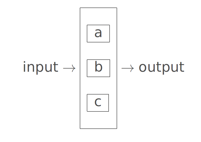
• To fix ideas, let’s assume that a system has three components: a, b, and c.

• Each component could be working or have failed.

• Define the events \[\begin{aligned} A &=\left\{ \text{Component a is working}\right\} \\ B &=\left\{ \text{Component b is working}\right\} \\ C &=\left\{ \text{Component c is working}\right\} \end{aligned}\]

Diagram of a system in serial

Components of a system may be arranged in series/sequential

Such a system fails when any one of the components fail.

Diagram of a system in parallel

Components of a system may be arranged in parallel

Such a system works when at least one of the components works.

System with independent components

Suppose events \(A,\) \(B\) and \(C\) are independent:

\[\begin{aligned} \mathbb{P}\left( A\cap B\cap C\right) &= \mathbb{P}\left( A\right) \, \mathbb{P}\left( B\right) \, \mathbb{P}\left( C\right) \\ & \\ \mathbb{P}\left( A\cap B\right) &= \mathbb{P}\left( A\right) \, \mathbb{P}\left( B\right) \\ & \\ \mathbb{P}\left( B\cap C\right) &= \mathbb{P}\left( B\right) \, \mathbb{P}\left( C\right) \\ & \\ \mathbb{P}\left( A\cap C\right) &= \mathbb{P}\left( A\right) \, \mathbb{P}\left( C\right) \end{aligned}\]

Components arranged in series

Suppose that \[ \mathbb{P}\left( A\right) = \mathbb{P}\left( B\right) = \mathbb{P}\left( C\right) =0.95.\] PROBLEM 1: Calculate the reliability of a serial system system. That is: \[P \left( \mbox{ system is working } \right)\]

Problem 1

• In serial systems, all the components need to be working for the system to work: \[W = \left\{ \text{System is working} \right\} = A\cap B\cap C\]

• Thus \[\begin{aligned} \mathbb{P}\left( W\right) &= \mathbb{P}\left( A\cap B\cap C\right) \\ & \\ &= \mathbb{P}\left( A\right) \, \mathbb{P}\left( B\right) \, \mathbb{P}\left( C\right) & \quad \text{ (independence)}\\ & \\ &=0.95^{3}\\ & \\ &=0.857 \end{aligned}\]

Problem 2

Calculate the reliability of a parallel system system.

• Systems with parallel components work if at least one their components works

• Thus \[\begin{aligned} W &=\left\{ \text{System\ is working}\right\} \\ & \\ &=A\cup B\cup C \\ & \\ &=\left( A^{c}\cap B^{c}\cap C^{c}\right)^{c} &\mbox{ (De Morgan)} \end{aligned}\]

Parallel independent components

Then

\[\begin{aligned} \mathbb{P}\left( W\right) &= \mathbb{P}\left[ \left( A^{c}\cap B^{c}\cap C^{c}\right) ^{c}\right] \\ & \\ &=1-\mathbb{P}\left( A^{c}\cap B^{c}\cap C^{c}\right) \\ & \\ &=1-\mathbb{P}\left( A^{c}\right) P\left( B^{c}\right) \, \mathbb{P}\left( C^{c}\right) & \quad \text{ independence} \\ & \\ &=1-\left( 1- \mathbb{P}\left( A\right) \right) \left( 1- \mathbb{P}\left( B\right) \right) \left( 1- \mathbb{P}\left( C\right) \right) \\ & \\ &=1-0.05^{3}\\ & \\ &\approx 0.9999. \end{aligned}\]

Combined systems

• Problem 3: Calculate the reliability of this combined system:

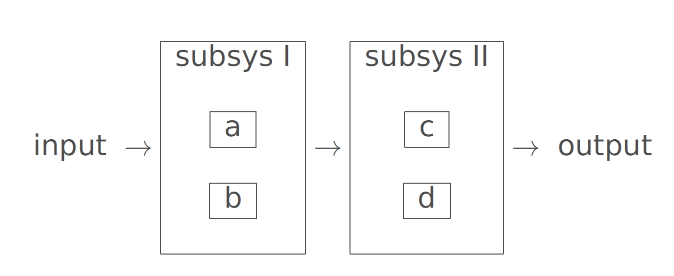
Combined system

• Assume that the components are independent and \[P\left( A\right) =P\left( B\right) =P\left( C\right) =P\left( D\right) =0.95.\]

Reliability of combined system

• In this case \[W=\left( A\cup B\right) \cap \left( C\cup D\right)\]

• One may verify that \(\left( A\cup B\right)\) and \(\left( C\cup D\right)\) are independent. Hint for the proof: it is sufficient to prove that \(A \cup B\) is independent of \(C\), and \(A \cup B\) is independent of \(D\).

• Therefore \[\begin{aligned} \mathbb{P}\left( W\right) &= \mathbb{P}\left( A\cup B\right) \, \mathbb{P}\left( C\cup D\right) &\quad \text{ independence} \\ & \\ &=\left( 2\times 0.95-0.95^{2}\right) \times \left( 2\times 0.95-0.95^{2}\right) \\ & \\ &=0.9950 \end{aligned}\]

Reliability of combined system

Alternatively:

\[\begin{aligned} \mathbb{P}\left( W\right) &= \mathbb{P}\left( A\cup B\right) \, \mathbb{P}\left( C\cup D\right) & \quad \text{ independence} \\ & \\ &=\left[ 1-\mathbb{P}\left( A^{c}\cap B^{c}\right) \right] \, \left[ 1-\mathbb{P}\left( C^{c}\cap D^{c}\right) \right] &\quad \text{ De Morgan \& compl.} \\ & \\ &=\left[ 1-\mathbb{P}\left( A^{c}\right) \, \mathbb{P}\left( B^{c}\right) \right] \left[ 1- \mathbb{P}\left( C^{c}\right) \, \mathbb{P}\left( D^{c}\right) \right] & \quad \text{ independence} \\ & \\ &=\left( 1-0.05^{2}\right) \left( 1-0.05^{2}\right) \\ & \\ &= 0.9950 \end{aligned}\]