Module 6

Continuous random variables

Matias Salibian Barrera

Last modified — 24 Oct 2025

Continuous random variables

• A random variable \(X\) is continuous if its CDF \(F_X(x) = \mathbb{P}(X \leq x)\) is continuous in \(x\).

• Stat 302 focuses on continuous random variables whose cdf can be written as \[F_X(x) = \mathbb{P}(X \leq x) = \int_{-\infty}^x f_X(t) \mathsf{d}t\] for some real function \(f_X\). Naturally, such \(f_X\) satisfies

  • \(f_X(a) \ge 0\) for all \(a \in \mathbb{R}\), and
  • \(\int_{-\infty}^{+\infty} f_X(t) \mathsf{d}t = 1\).

• We say that \(f_X\) is the probability density function (PDF) of \(X\).

Continuous random variables

• Recall that CDFs are always right-continuous \[F_X(a) \, = \, \lim_{u \searrow a} F_X(u) \qquad \forall \, a \in {\mathbb{R}}\] where “\(u \searrow a\)” means taking the limit with \(u > a\)

• For continuous random variables, the CDF is continuous, so the left- and right-limits coincide: \[F_X(a) \, = \, \lim_{u \searrow a} F_X(u) \, = \, \lim_{u \nearrow a} F_X(u) \, = \, \lim_{u \to a} F_X(u) \, , \quad \forall \, a \in \mathbb{R}\]

Continuous random variables

If \(X\) is continuous with CDF and PDF \(F_X(x)\) and \(f_X(x)\), then

• \(\mathbb{P}( a < X \le b ) \, = \, F_X(b) - F_X(a) = \int_a^b \, f_X(t) \, \mathsf{d}t\)

• \(\mathbb{P}(a < X < b) = \mathbb{P}(a \leq X < b) = \mathbb{P}(a < X \leq b) = \mathbb{P}( a \le X \le b )\)

• For any \(a \in \mathbb{R}\) we have \(\mathbb{P}(X = a) = 0\)

Expectation formula of a continuous \(X\)

Let \(X\) be continuous with cdf and pdf \(F_X(x)\) and \(f_X(x)\).

• If \(g : {\mathbb{R}}\to {\mathbb{R}}\), then

\[ \mathbb{E}[g ( X )]= \int_{-\infty }^{\infty } g(t) f_X(t) \, \mathsf{d}t \]

if the integral exists.

• In particular:

\[\mathbb{E}[ X ] \, = \, \int_{-\infty }^{\infty } \, t \, f_X(t)\, \mathsf{d}t.\]

Often \(f_X(t) = 0\) outside some interval \([a, b]\). If so, the integrals above can naturally be restricted to the interval \([a, b]\)

Variance of \(X\)

• As before, the variance of \(X\) is \[\operatorname{Var}(X) = \mathbb{E}[ (X - \mathbb{E}[X])^2] =\mathbb{E}[X^{2}] - (\mathbb{E}[X])^{2}\]

The proof is similar as for the discrete case, but now we use integrals instead of sums. To simplify the notation, call \(\mu_X = \mathbb{E}[X]\):

\[\begin{aligned} \operatorname{Var}(X) &=\int_{-\infty}^\infty (a-\mu_X)^{2} \, f_X(a) \, \mathsf{d}a = \int_{-\infty}^\infty (a^{2} + \mu_X^{2} - 2 \, a) \, f_X(a) \, \mathsf{d}a \\ & \\ &= \int_{-\infty }^{\infty} a^{2} \, f_X(a) \, \mathsf{d}a + \mu_X^{2} \overset{1}{\overbrace{\int_{-\infty }^{\infty}f_X(a) \, \mathsf{d}a}} - 2 \, \mu_X \, \overset{\mu_X}{\overbrace{\int_{-\infty }^{\infty} a \, f_X(a) \, \mathsf{d}a}} \\ & \\ &= \mathbb{E}[X^{2}] - \mu_X^{2} = \mathbb{E}[X^{2}] - (\mathbb{E}[X])^{2} \end{aligned} \]

Observations

• The density function \(f_X(x)\) may be larger than 1!

• \(f_X(a) \ne \mathbb{P}( X = a )\)

• Because of the Fundamental Theorem of Calculus:

\[ F_X'(a) = \left. \frac{\mathsf{d}}{\mathsf{d}x} F_X \left( x \right) \right|_{x = a}\, = \, \left. \frac{\mathsf{d}}{\mathsf{d}x} \left[ \int_{-\infty}^x f_X(t) \, \mathsf{d}t \right] \right|_{x=a} \, = \, f_X(a) \]

we have

\[ f_X(x) = \lim_{ \delta \to 0+} \frac{\mathbb{P}(X \leq x+\delta) - \mathbb{P}(X\leq x)}{\delta} \]

• As in the discrete case, given the PMF we can obtain the CDF, and given the CDF, we can obtain the PMF

Interpreting density functions

• Intuitively, regions with (relatively) higher values of \(f_X\) have higher probability

• Because, for very small values of \(\delta > 0\)

\[ \mathbb{P}\left( x - \delta/2 < X < x + \delta/2 \right) \ = \ \int_{x-\delta /2}^{x+\delta/2} f_X\left( t\right) \mathsf{d}t \quad \approx \quad f_X(x) \delta \]

Computations for discrete and continuous rv’s

• Where we used sums for discrete distributions, we use integrals in the case of continuous ones

\[\begin{aligned} && \text{Discrete} && \text{Continuous} \\ F(x) && \sum_{k\leq x} f\left( k\right) && \int_{-\infty}^{x}f\left( t\right) \mathsf{d}t \\ & & \\ \mathbb{E}[ g(x) ] && \sum_{i \in {\cal R}_X} g\left( i\right) f\left( i\right) && \int_{-\infty }^{\infty } g\left( u\right) f\left( u\right) \mathsf{d}u\\ & & \\ \mathbb{P}( X\in B ) && \sum_{h\in B}f ( h ) && \int_{B} f(a) \mathsf{d}a \end{aligned} \]

• Recall that \(f_X(t) = 0\) for \(t \notin {\cal R}_X\).

Uniform distribution

• For \(a < b\), real numbers, the \({\mathrm{Unif}}(a, b)\) distribution has density function \[f_X(x) \, = \, \begin{cases} 0 & x < a \\ 1 / \left( b - a \right) & a \le x \le b \\ 0 & x > b \end{cases}\]

• More concisely:

\[ f_X \left( x \right) \, = \, \frac{1}{ \left( b - a \right)} \, \mathbf{1}_{(a, b)}(x) \] where \(\mathbf{1}_H(x)\) is the indicator function of the set \(H\):

\[ \mathbf{1}_H(x) = 1 \ \ \text{ if } \ x \in H\, , \quad \text{ and } \quad \mathbf{1}_H(x) = 0 \ \ \text{ if } \ \ x \notin H \]

Uniform distribution

• The CDF of a random variable with a \({\cal U}(a, b)\) distribution is

\[ F_X \left( x \right) \, = \, \begin{cases} 0 & x \le a \\ \frac{x - a} {b - a} & a < x < b \\ 1 & x \ge b \end{cases} \]

• For \(a \le s < t \le b\) we have

\[ \mathbb{P}\left( s < X \le t \right) = \mathbb{P}\left( s < X < t \right) = \mathbb{P}\left( s \le X \le t \right) = F_X(t) - F_X(s) = \frac{t - s}{b - a} \]

(hence the name uniform)

Uniform distribution

• However, for regions that go outside the range \({\cal R}_X = [a, b]\), things are a bit more delicate:

• If \(t > b\) (but \(a \le s\)):

\[ \begin{aligned} \mathbb{P}\left( s < X \le t \right) = \mathbb{P}\left( s < X < t \right) = \mathbb{P}( s \le X \le t ) \, & = \, F(t) - F(s) \\ & = 1 - F(s)\\ &= \frac{b - s}{b - a}. \end{aligned} \]

• Similarly, if \(s < a\) (but \(t \le b\)):

\[ \mathbb{P}\left( s < X \le t \right) = \mathbb{P}\left( s < X < t \right) = \mathbb{P}\left( s \le X \le t \right) = \frac{t - a}{b - a} \]

Distribution family

• For different values of \(a < b\) we get different uniform distributions

• It is useful to study families of distributions, since many of their properties hold across all members of the family.

• For example, if the random variable \(X\) has a Binomial distribution, \(Bin(n, p)\), regardless of the actual values of \(n \in \mathbb{N}\) and \(p \in [0, 1]\), we always have \(\mathbb{E}[X] = n \, p\) and \(V(X) = n \, p \, (1-p)\)

• If \(X \sim {\mathrm{Unif}}(a, b)\)

\[ \begin{aligned} \mathbb{E}\left[ X\right] & = \int_{-\infty}^{+\infty} t \, f_X(t) \, \mathsf{d}t = \int_a^b t \, f_X(t) \, \mathsf{d}t = \int_a^b t \, \left( \frac{1}{b - a} \right) \, \mathsf{d}t \\ &= \frac{1}{b-a} \, \int_a^b t\, \mathsf{d}t = \left( \frac{1}{b - a} \right) \, \left[ \left. \frac{x^{2}}{2}\right\vert _{a}^{b} \right] \\ &=\frac{1}{b-a} \, \left( \frac{b^2-a^2}{2} \right) =\frac{a + b}{2} \end{aligned}\]

Variance of a Uniform random variable

• Check that if \(X \sim {\cal U}(a, b)\) then

\[ \mathbb{E}\left[ X^2 \right] \, = \, \frac{b^{3}-a^{3}}{3\left( b - a \right) } \, = \, \frac{b^{2}+a^{2}+ a \, b }{3} \]

And thus, for any \(a < b\), we have that if \(X \sim {\cal U}(a, b)\)

\[ \operatorname{Var}(X) = \mathbb{E}\left[ X^2 \right] - \left( \mathbb{E}\left[ X \right] \right)^2 = \frac{ \left(b - a \right)^2 }{ 12 }\]

The expectation and variance formulas are applicable to all distributions in the continuous uniform distribution family.

Calculating uniform probabilities

Suppose that \(X\sim{\mathrm{Unif}}( 0, 10)\)

Calculate

1. \(\mathbb{P}\left( X>3\right)\).
2. \(\mathbb{P}\left( 2\leq X<12\right)\).
3. \(\mathbb{P}\left( X>5 \ \vert\ X>2\right)\).

Solution

1. Because \(X\) has a uniform distribution with parameters 0 and 10, we have: \(F_X\left( a\right) =\frac{a}{10}\) for \(0 \le a \le 10\), \(F_X(a) = 0\) for \(a < 0\) and \(F_X(a) = 1\) for \(10 \le a\). Thus

\[ \mathbb{P}\left( X > 3\right) = 1 - F_X\left( 3\right) = 1-\frac{3}{10}=0.70 \]

2. Because \(12 > 10\) (the upper limit of the support of \(f_X\)), \(F_X(12) = 1\), thus: \[ \mathbb{P}\left( 2\le X < 12\right) = F_X\left( 12 \right) -F_X\left( 2\right) =1-\frac{2}{10}=0.80 \]

Solution (cont’d)

3. Using the definition of conditional probability: \[ \begin{aligned} \mathbb{P}\left( X>5 \ \vert\ X>2\right) &=\frac{\mathbb{P}\left( \{X>5\} \cap \{X>2\} \right) }{\mathbb{P}\left( X>2\right) } \\ &=\frac{\mathbb{P}\left( X>5\right) }{\mathbb{P}\left( X>2\right) } = \frac{1-F_X\left( 5\right) }{1-F_X\left( 2\right) } \\ &=\frac{1-\left( 5/10\right) }{1-\left( 2/10\right) } = \frac{(5/10)}{(8/10)} = 5/8 = 0.625 \end{aligned} \]

In the second line above we used that since \(\{ X > 5 \} \subseteq \{ X > 2 \}\), we have \[ \{ X > 5 \} \cap \{ X > 2 \} = \{ X > 5 \} \]

Functions of continuous r.v.’s

Consider a continuous random variable \(X\) and define a new random variable \[Y \, = \, g \left( X \right)\] where \(g : \mathcal{R}_X \to {\mathbb{R}}\).

• Expected value:

\[ \mathbb{E}\left[ Y \right] = \mathbb{E}[ g(X) ] = \int_{-\infty }^{\infty }g\left( x\right) f_X \left( x\right) \mathsf{d}x \]

(this is neither obvious, nor easy to prove)

Expected values of functions of random variables

• Let \(X \thicksim {\cal U} (0, 1)\) and \(Y = 1 / (X + 1)\). What is \(\mathbb{E}\left[ Y \right]\)?

 

• We have: \(f_X(x) = 1\) for \(x \in [0,1]\), and \(f_X(x) = 0\) elsewhere.

 

• With \(g(x) = 1/(x+1)\), we have

\[ \mathbb{E}\left[ Y\right] = \mathbb{E}\left[ \frac{1}{X+1}\right] =\int_{-\infty }^{\infty } g(a) f_X(a) \mathsf{d}a = \int_{0}^{1} \left( \frac{1}{a+1} \right) \mathsf{d}a =\log \left( a+1\right) \bigg|_{0}^{1} = \, \log(2) \]

Expectation of transformations again

• Consider a stick of length one (unit)

• The stick has a mark at location \(x_0 \in [0, 1]\)

• We break the stick in two pieces at a random location \(X \sim {\mathrm{Unif}}(0,1)\) along it

• Let \(Y\) be the length of the piece that contains the mark

1. Calculate \(\mathbb{E}\left[ Y \right]\)
2. Which value of \(x_0\) maximizes \(\mathbb{E}\left[ Y \right]\)?

Solution \(\mathbb{E}\left[ Y \right]\)

• The stick is broken at the point \(X\).

• Either \(X < x_0\) or \(X \ge x_0\). Then:

  1. If \(X < x_0\) then \(Y = 1 - X\),
  2. If \(X \ge x_0\) then \(Y = X\).

• Therefore

\[ Y = g \left( X \right) \, = \, \begin{cases} 1 - X & X < x_0; \\ X & X \ge x_0. \end{cases} \]

\[ \begin{aligned} \mathbb{E}\left[ Y\right] &= \int_{-\infty }^{\infty }g\left( x\right) f\left( x\right) \mathsf{d}x=\int_{0}^{1}g\left( x\right) \mathsf{d}x =\int_{0}^{x_0}\left( 1-x\right) \mathsf{d}x + \int_{x_0}^{1}x\mathsf{d}x \\ &=\frac{1}{2}+x_0-x_0^{2} =\frac{1}{2}+x_0\left( 1-x_0\right). \end{aligned} \]

Solution: Which value of \(x_0\) maximizes \(\mathbb{E}\left[ Y \right]\)?

Define \(h(x_0) = \mathbb{E}[{Y}] = 1/2 + x_0 (1-x_0 )\) and notice that this function is at least twice continuously differentiable.

It extrema will satisfy the first order condition:

\[ \frac{\mathsf{d}}{\mathsf{d}x_0} h(x_0) = 1 - 2x_0 \overset{set}{=} 0 \quad \Longleftrightarrow \quad x_0 = 1/2 \]

• Since \(\frac{\mathsf{d}^2}{\mathsf{d}x^2_0}h(x_0) = -2 < 0\) for all \(x_0 \in (0,1)\), then the above critical point \(x_0= 1/2\) is the unique maximum

CDF and PDF of functions of a random variable

• If \(X\) is a random variable and \(Y = g(X)\) for some function \(g(\cdot)\), then we want to find the relationship between the CDF’s of the 2 random variables: \(F_Y\) and \(F_X\)

• Standard procedure:

  • Find the range of \(Y\): \(\mathcal{R}_Y\).

  • Calculate the CDF \(F_Y(y)\) for \(y \in \mathcal{R}_Y\):

  \[ F_Y(y) = \mathbb{P}\left( Y \le y \right) = \mathbb{P}\left( g \left( X \right) \le y \right) \]

• Then find its PDF by taking derivative of the CDF:

\[ f_Y(y) = F'_Y(y) \]

Example

Let \(X \sim {\mathrm{Unif}}\left( -1,1\right)\)

Find the CDF and PDF of:

1. \(Y = X^3\)
   
2. \(Z = X^2\)

Recall that

• The PDF of \(X\) is \[f_X(x) = \begin{cases}\frac{1}{2} & x \in (-1, 1)\\ 0 & x \notin (-1, 1).\end{cases}\]

• The CDF of \(X\) is \[F_X(x) = \begin{cases} 0 & x < -1\\ \displaystyle \frac{x+1}{2} & x \in (-1, 1)\\ 1 & x > 1.\end{cases}\]

Solution for \(Y = X^3\)

• The range of \(Y = X^3\) is \(\mathcal{R}_Y = (-1, 1)\).

• Hence: \(F_Y(y) = 0\) if \(y < -1\), and \(F_Y(y) = 1\) if \(y > 1\).

• For \(y \in (-1, 1)\) we have \[\begin{aligned} F_y(y) & = \mathbb{P}( Y \le y ) = \mathbb{P}( X^3 \le y ) \\ &= \mathbb{P}( X \le y^{1/3} ) = \int_{-1}^{y^{1/3}} (1/2) \, \mathsf{d}t \\ & = ( y^{1/3} + 1 ) / 2. \end{aligned}\]

• Sanity check: \(F_Y\) should be continuous: \(F_Y(-1) = 0\), \(F_Y(1) = 1\).

• The PDF of \(Y\), \(f_Y(y) = F_Y'(y) = \frac{1}{2} \times \frac{1}{3} \times y^{1/3 - 1} = \frac{1}{6} \, y^{-2/3}\) for \(y \in (-1, 1)\), thus:

\[ f_Y(y) = F_Y'(y) = \begin{cases} 0 & y \notin (-1, 1) \\ \displaystyle \frac{y^{-2/3}} {6} & y \in (-1, 1), \end{cases}\]

Note that \(f_Y(0)\) is not defined, but still \(\int_{-1}^1 f_Y(y) \mathsf{d}y = \left. (1/2) y^{1/3} \right|_{-1}^1 = 1\)

Solution for \(Z = X^2\)

• Here \(\mathcal{R}_Z = [0, 1]\).

• Thus: \(F_Z(z) = 0\) for \(z < 0\) and \(F_Z(z)=1\) for \(z > 1\).

• For \(z \in (0, 1)\)

\[\begin{aligned} F_Z(z) &= \mathbb{P}(Z \leq z) = \mathbb{P}(X^2 \leq z) = \mathbb{P}(-\sqrt{z} \leq X \leq \sqrt{z}) \\ &= \int_{-\sqrt{z}}^{\sqrt{z}} (1/2) \mathsf{d}t = (1/2) \left( \Bigl. t \ \Bigr|_{-\sqrt{z}}^{\sqrt{z}} \right) = (1/2) \left( \sqrt{z} - (-\sqrt{z}) \right) = \sqrt{z} \end{aligned}\]

• Sanity check: we can see that \(F_Z\) is continuous (\(F_Z(0) = 0\), \(F_Z(1)=1\)), and non-decreasing.

• For the PDF: \(f_Z(a) = 0\) if \(a \notin (0, 1)\) and \[ f_Z(a) = F_Z'(a) = \frac{1}{2} a^{-1/2} = \frac{1}{2 \, \sqrt{a}} \quad \text{ for } a \in (0, 1) \]

Example

• Let \(X \sim {\mathrm{Unif}}(0,1)\) and \(Y = - \log(X)\), where \(\log( \cdot )\) is the natural logarithm function.

• Find the cdf and pdf of \(Y\): \(F_Y\) and \(f_y\).

Solution:

Exponential distribution

• Waiting times are usually modeled using an exponential distribution.

Examples: the time until

• a new customer arrives
• an earthquake occurs
• a network crashes
• a system component fails

Mathematical definition

Definition

We say that \(X \sim {\cal E}(\lambda)\) follows the exponential distribution with parameter \(\lambda > 0\) if

\[ F_X(x) = \begin{cases} 1 - e^{-\lambda \, x} & \text{ if } x > 0 \\ & \\ 0 & \text{otherwise} \end{cases} \]

• If the CDF of a random variable \(W\) is \[ F_W(t) = 1 - e^{-3.5 \, t} \qquad \text{ for } t \ge 0 \] and \(F(t) = 0\) for \(t < 0\), then \(W \sim {\cal E}(3.5)\)

• Last example revisited: if \(X \sim {\cal U}(0,1)\) and \(Y = -\log(X)\), then what is the distribution of \(Y\)? \(Y \ \sim \ ???\)

Exponential distribution family

• This leads to the family of exponential distributions \({\cal E}(\lambda)\), where \(\lambda > 0\) is a fixed arbitrary positive real number.

• We have already encountered several families of distributions:

  • the Uniform family \({\cal U}(a, b)\), where \(a < b\)
  • the Binomial family \(Bin(n, p)\) with \((n, p) \in \mathbb{N} \times [0, 1]\)
  • The Poisson family \({\cal P}(\lambda)\), \(\lambda > 0\)
  • The Geometric family \(Geom(p)\) with \(p \in (0, 1)\)
  • etc.

• The set of possible values of the unknown parameters (for example: \(\lambda\), or \((n, p)\), or \((a, b)\) with \(a < b\), etc.) is called the parameter space

Exponential distribution

• The PDF is \[f_X(x) = F_X'(x) = \begin{cases}\lambda \, e^{-\lambda \, x} & \text{ if } x > 0\\ 0 & \text{otherwise}\end{cases}\]

• There is a connection between the Exponential distribution and the Poisson distribution. We will see that if \(X \sim {\cal P}(\lambda)\), then the (random) wait time \(T\) until the next occurrence of the event that \(X\) counts satisfies \(T \sim {\cal E}(\lambda)\).

• Thus, \(\lambda\) is typically said to represent the rate of occurrence of the event being modeled. For example:
  \[\begin{aligned} \lambda & = 5 \text{ customers per hour} \\ \lambda & = 0.5 \text{ earthquakes per year} \end{aligned}\]

Mean and variance

• If \(X \sim {\cal E}(\lambda)\) for some \(\lambda > 0\), then

\[\mathbb{E}[ X ] \, = \, \int_{-\infty}^{\infty} t \, f_X(t) \, \mathsf{d}t \, = \, \int_0^{\infty} t \, \lambda \, e^{-\lambda \, t} \, \mathsf{d}t \, = \, 1/ \lambda \]

• Simple integration (do it!) gives \(\mathbb{E}[ X^2 ] \, = \, 2/\lambda^2\) and hence \(\operatorname{Var}(X) = 1/\lambda^2 = (\mathbb{E}[X])^2\)

Warning

Different textbooks and software use different parametrizations of the Exponential distribution.

• “Rate” parameterization is what we defined.
• “Mean” parameterization defines the PDF \(f_X(x) = \frac{1}{\delta}e^{-x/\delta}\mathbf{1}_{(0, \infty)}(x)\) so that \(\mathbb{E}[X] = \delta\) (equal the parameter, rather than “1 over the parameter” as in our case)
• It does not matter which parametrization you use, as long as you remain consistent

Exponential and Poisson connection

• Let \(X\) be the number of events occurring in a unit of time

 

• Suppose that \(X\) follows a Poisson distribution with rate \(\lambda > 0\) per unit of time

 

• Let \(T\) be the (random) waiting time (in the same time units) between events

 

• Then we will show that \[T \ \sim \ {\cal E}( \lambda )\]

We will find the CDF of \(T\): \(F_T(t)\) for \(t \in \mathbb{R}\)

Exponential and Poisson connection

• Fix \(t > 0\), and let \(X_t\) be the number of events in the next \(t\) units of time, then

\[ X_t \sim {\cal P}( \lambda \, t) \]

• Also \(\{ T > t \} = \{ X_t = 0 \}\) (why?) thus \[ \mathbb{P}( T>t) = \mathbb{P}( X_t=0) = \frac{e^{-\lambda t}( \lambda t)^{0}}{0!} = e^{-\lambda t} \]

• Hence: \[ F_T(t) = \mathbb{P}( T \leq t ) = 1 - \mathbb{P}( T > t) = 1 - e^{-\lambda t} \qquad \text{ for } t > 0 \]

Exponential and Poisson connection (cont’d)

• For \(t < 0\), note that \(\mathbb{P}\left( T \leq t \right) = 0\), so \[ F_T(t) = \left\{ \begin{array}{ll} 1 - e^{-\lambda t} & \text{ if } t > 0 \\ 0 & \text{ if } t \le 0 \end{array} \right. \] which is the CDF of an \({\cal E}(\lambda)\) distribution

Exercise

Suppose that cases of an infectious disease in BC follow a Poisson process with rate \(\lambda =3\) per 30 days. In other words, the number of cases in any 1-month period is a random variable \(C\) with \(C \sim {\cal P}(3)\).

1. What is the probability that the first case in October will occur after October 15th?
2. Conditional of having no cases in the first 10 days of October, what is the probability that the first case in October occurs before October 20th?

Solution

• Let \(X\) be the number of cases per day, then \(X \sim {\cal P}( 3/30 ) = {\cal P}( 1/10 )\)

• Let \(T\) be the waiting time (in days) until the first outbreak in October. Then \(T \sim {\cal E}(1/10)\)

• The question asks for \(\mathbb{P}( T \ge 15)\), so: \[\begin{aligned} \mathbb{P}( T \ge 15 ) = 1 - \mathbb{P}( T \le 15 ) & = 1 - \int_{0}^{15} 0.1 \, e^{-0.1 \, t} \, \mathsf{d}t \\ & \\ &=e^{-1.5} \ \approx \ 0.22313 \end{aligned}\]

Solution b. No outbreak so far, outbreak after 20th.

• For part (b), the conditioning event is that \(T > 10\).

• We need to calculate \(\mathbb{P}( T \le 20 | T > 10)\): \[\begin{aligned} \mathbb{P}( T < 20 \ \vert\ T > 10 ) &=\frac{ \mathbb{P}( \{ T<20 \} \cap \{ T>10 \} ) }{\mathbb{P}( T>10 ) } = \frac{\mathbb{P}( 10<T<20\ ) }{\mathbb{P}( T>10\ ) } \\ & \\ &= \frac{F_{T}( 20 ) - F_T ( 10 ) }{1 - F_T ( 10 ) } \\ & \\ &= \frac{e^{-0.1\times 10}-e^{-0.1\times 20}}{e^{-0.1\times 10}} = 1 - e^{-0.1\times 10} \\ & \\ &= \mathbb{P}(T < 10) \end{aligned}\]

“Memoryless”

• Let \(W \sim {\cal E}(\lambda)\), for some \(\lambda > 0\).

• To fix ideas, assume that \(W\) is the lifetime of a system (the time until the system fails)

 

• Let us compare

\[ \mathbb{P}( W > h ) \qquad \text{and} \qquad \mathbb{P}(W > t + h \ \vert\ W > t ) \]

 

• The first is the probability that the system works for at least \(h\) more years

 

• The second is [the conditional probability that the system works for at least \(h\) more years conditional on having worked for at least \(t\) years

“Memoryless”

• We have

\[ \mathbb{P}( W > h ) = 1 - \mathbb{P}( W \le h) = e^{-\lambda \, h} \]

• Also

\[ \begin{aligned} \mathbb{P}(W > t+h \ \vert\ W> t ) &= \frac{\mathbb{P}\left( \left\{ W>t+h \right\} \cap \left\{ W > t \right\} \right) } {\mathbb{P}\left( W>t \right) } \\ &=\frac{\mathbb{P}\left( W>t+h \right) }{\mathbb{P}\left( W>t \right) } \\ &= \frac{e^{-\lambda \,( t+h) } }{e^{-\lambda \, t}} = e^{-\lambda \, h} = \mathbb{P}\left( X > h \right) \end{aligned} \] (regardless of \(t\))

Implications of the memoryless property

If this model is appropriate

• At age \(t\), the probability of surviving until age \(t+h\) is the same for any \(t\)

• E.g. the probability of reaching 35 at age 30 is the same as that of reaching 95 at age 90

• In other words: the system does not “get old”

• This may not always be realistic (people?)

• Model choices may have unintended consequences

The Normal (Gaussian) distribution

Definition

A random variable \(Z\) is said to have a standard normal distribution, denoted as \(\mathcal{N}(0, 1)\) its PDF is given by \[f_Z(z) = \phi (z) = \frac{1}{\sqrt{2\pi }} \exp(-z^{2}/2) \, , \quad z \in {\mathbb{R}}\]

• The CDF \(F_Z(z)\) is

\[ F_Z(z) = \Phi (z) \, = \, \int_{-\infty }^{z}\phi(t) \, dt \, = \, \int_{-\infty }^{z} \frac{1}{\sqrt{2\pi }} \exp(-t^{2}/2) \, dt \]

• There is no explicit formula for this CDF \(\Phi\)

The Normal (Gaussian) distribution

• The value of \(\Phi (z)\) has to be computed numerically

• In the old days, people used tables:

\(z\)	\(\Phi (z)\)	\(z\)	\(\Phi (z)\)
1.645	0.950	-1.645	0.050
1.960	0.975	-1.960	0.025
2.326	0.990	-2.326	0.010
2.576	0.995	-2.576	0.005

• Now of course we use computers

The Normal (Gaussian) distribution

• The Standard Normal distribution is symmetric around 0:

\[ \phi(z) = \phi(-z) \quad \text{for any } z \in \mathbb{R} \]

• This implies

\[ \Phi(a) = \mathbb{P}( Z \le a) = \mathbb{P}( Z \ge -a) = 1 - \Phi(-a) \qquad \forall \, a \in {\mathbb{R}} \]

Symmetry

Mean of Normal distribution

• The mean of a standard normal random variable is \(\mathbb{E}[ Z ]=0\).

• Proof: if \(\phi(z)\) is the density of \(Z\), then \[\phi'(z) \, = \, -z \, \phi(z) \qquad \mbox{ (prove it!)}\] and thus

\[ \begin{aligned} \mathbb{E}[ Z ] & = \int_{-\infty}^\infty z \, \phi (z) \, \mathsf{d}z \, = \, - \int_{-\infty}^\infty \phi'(z) \, \mathsf{d}z = \lim_{u \to \infty} \bigg(\phi(u) - \phi(-u)\bigg) = 0. \end{aligned} \]

Variance of Normal distribution

• The variance of standard normal is \(\operatorname{Var}( Z ) =1\):

\[\begin{aligned} \operatorname{Var}(Z)&= \mathbb{E}[ Z^{2}] =\int_{-\infty }^{\infty }z^{2}\phi (z)\mathsf{d}z =2\int_{0}^{\infty }z^{2}\phi (z)\mathsf{d}z =-2\int_{0}^{\infty }z\phi ^{\prime }(z)\mathsf{d}z. \end{aligned}\]

Integration by parts with \[\begin{aligned} u &=z & \mathsf{d}v&=\phi ^{\prime }(z)\mathsf{d}z \\ \mathsf{d}u &=\mathsf{d}z & v &= \phi (z) \end{aligned}\] gives \[ \operatorname{Var}\left( Z\right) = -2\biggl[ \quad \overset{0}{\overbrace{z\phi (z)\bigg|_{0}^{\infty }}} -\overset{1/2}{\overbrace{\int_{0}^{\infty }\phi (z)dz}}\quad \biggr] =1.\]

Notation/terminology

• \(Z \thicksim N(0, 1)\) means

  \(Z\) is a Gaussian (Normal) random variable with mean 0 and variance 1.

• Equivalently:

  \(Z\) is a standard normal random variable

Gaussian (Normal) random variables

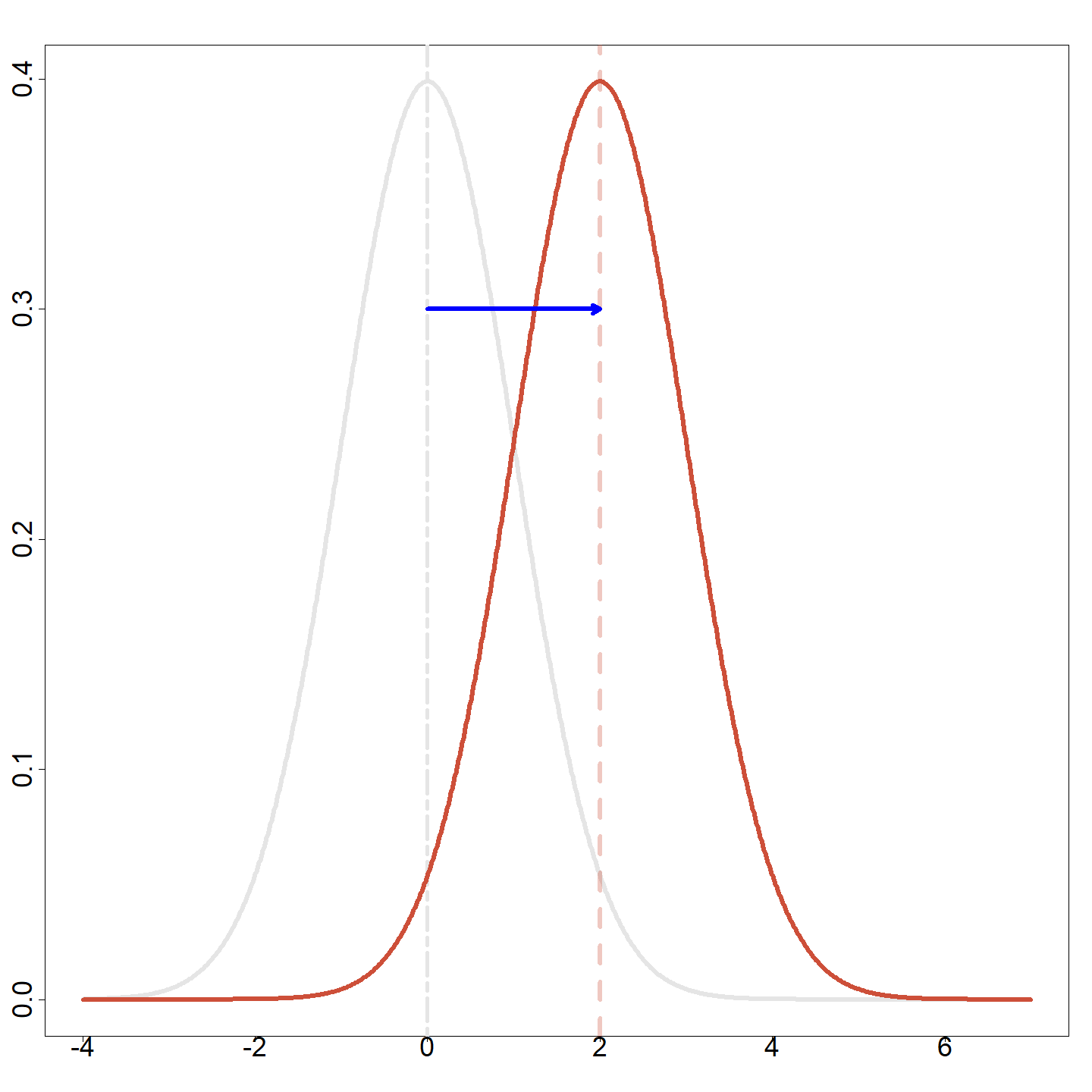
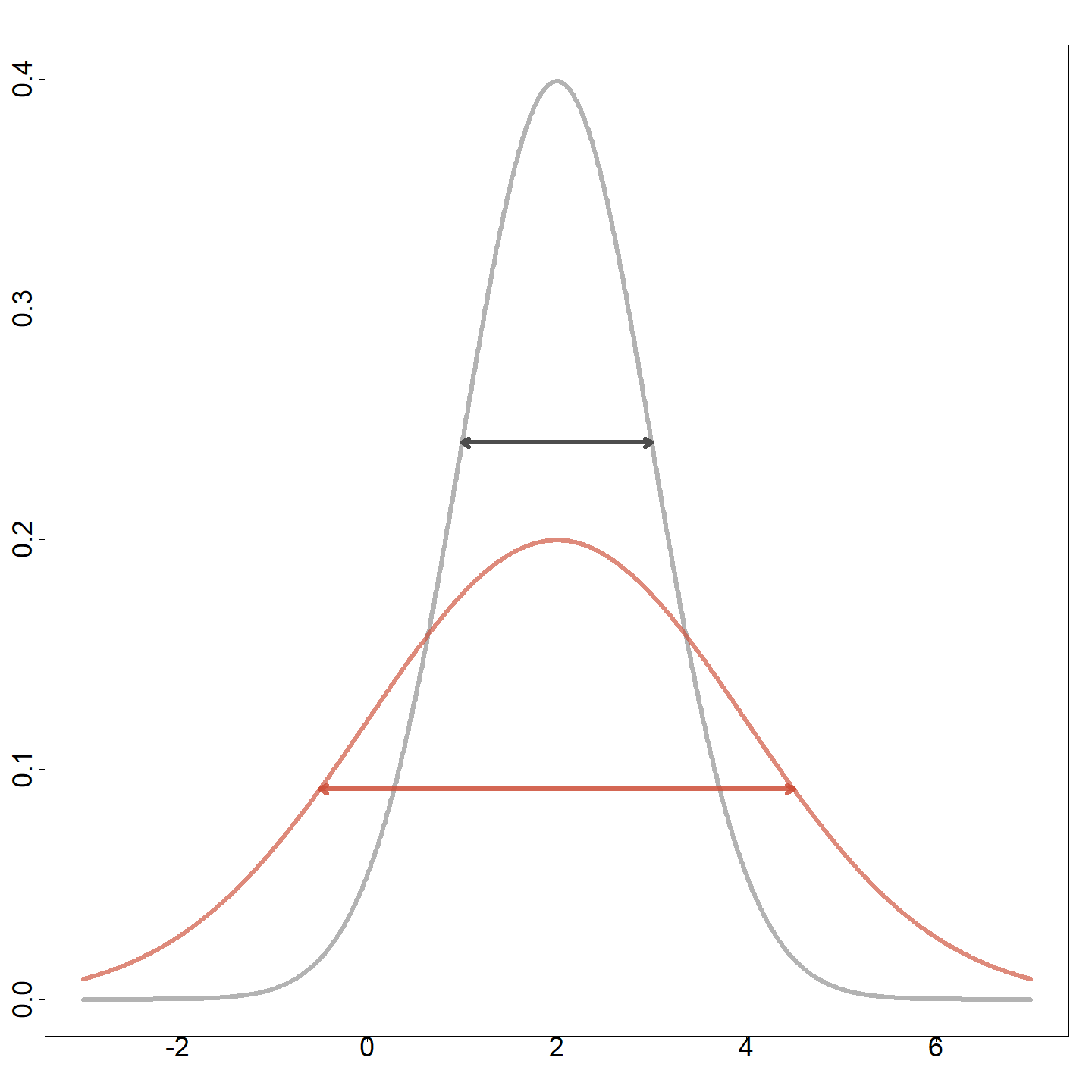
• Let \(Z\sim \mathcal{N}\left( 0,1\right)\) and, for \(\mu \in {\mathbb{R}}\), \(\sigma > 0\), define \[X=\mu +\sigma Z\]

• We say \(X\) has a Gaussian distribution, and we have \[\begin{aligned} \mathbb{E}\left[ X\right] &=\mathbb{E}\left( \mu +\sigma Z\right) = \mu +\sigma \overset{0}{\text{ }\overbrace{E\left( Z\right) }}\text{ }=\mu;\\ \operatorname{Var}(X) &= \operatorname{Var}\left( \mu +\sigma Z\right) =\sigma ^{2}\overset{1}{ \text{ }\overbrace{Var\left[ Z\right] }}\text{ }=\sigma ^{2}.\end{aligned}\]

• Notation: \(X \sim \mathcal{N}\left( \mu ,\sigma^2 \right)\).

The pdf and cdf of Gaussian rv (Normal)

The cdf of \(X\sim\mathcal{N}(\mu,\sigma^2)\) is \[\begin{aligned} F_X\left( x\right) &= \mathbb{P}\left( X\leq x\right) = \mathbb{P}\left( \frac{X-\mu }{\sigma } \leq \frac{x-\mu }{\sigma }\right) = \mathbb{P}\left( Z\leq \frac{x-\mu }{\sigma }\right) =\Phi \left( \frac{x-\mu }{\sigma }\right). \end{aligned}\]

Its pdf is given by \[\begin{aligned} f_X\left( x\right) &= F_X^{\prime }\left( x\right) =\frac{1}{\sigma }\phi \left( \frac{x-\mu }{\sigma }\right) = \frac{1}{\sigma \sqrt{2\pi }} \exp \Big \{ -\frac{1}{2}\left( \frac{x-\mu }{\sigma} \right)^{2} \Big \}. \end{aligned}\]

Warning

Often, \(Z\) is used specifically for standard normal RV’s

Different means

Different variances

Computing Gaussian probabilities

• The following key result can be used to compute probabilities for a Gaussian distribution with any mean and any variance: \[X \thicksim \mathcal{N}\left( \mu ,\sigma ^{2}\right) \ \Longleftrightarrow \ Z = \frac{X - \mu}{\sigma} \thicksim N\left( 0, 1 \right)\] hence \[\mathbb{P}\left( X \le t \right) \, = \, F_X(t) \, = \, \Phi \left( \frac{t-\mu }{\sigma }\right)\] where \(\Phi\) is the cdf of a standard normal distribution. In other words, one only needs to be able to compute one cdf (namely: \(\Phi\))

• Very good numerical approximations exist to compute the function \(\Phi\)

Exercise: Calculating normal probabilities

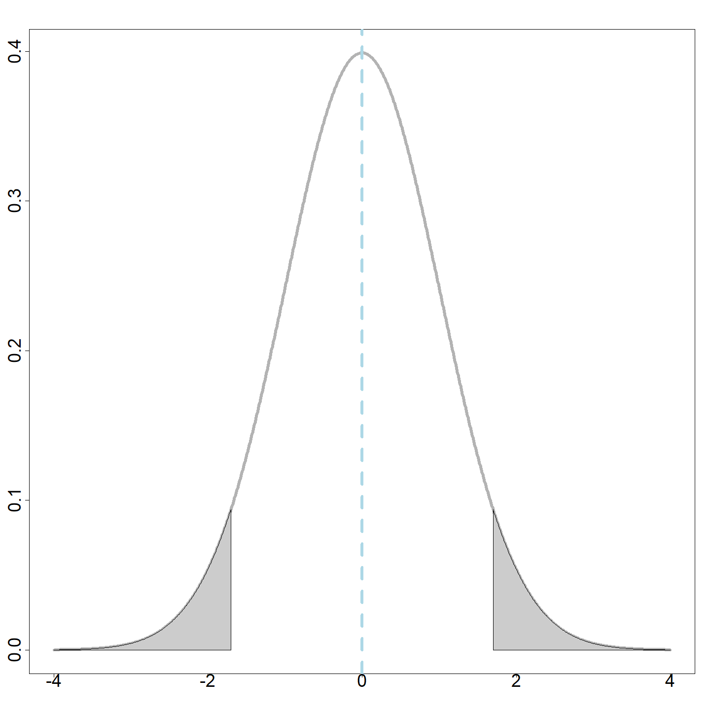
Let \(Z\sim \mathcal{N}\left( 0,1\right)\). Calculate  

1. \(\mathbb{P}\left( 0.10\leq Z\leq 0.35\right)\).

2. \(\mathbb{P}\left( Z>1.25\right)\).

3. \(\mathbb{P}\left( Z>-1.20\right)\).

4. Find \(c\) such that \(\mathbb{P}\left( Z>c\right) =0.05\).

5. Find \(c\) such that \(\mathbb{P}\left( \left\vert Z\right\vert <c\right) =0.95\).

We will use R to demonstrate.

a. \(\mathbb{P}\left( 0.10\leq Z\leq 0.35\right)\)

We have \[\begin{aligned} \ P\left( 0.10\leq Z\leq 0.35\right) &= \Phi \left( 0.35\right) -\Phi \left( 0.10\right) \approx 0.097. \end{aligned}\]

``` r
pnorm(0.35) - pnorm(0.10)
```

``` julia
using Distributions;
cdf(Normal(), 0.35) - cdf(Normal(), 0.10)
```

``` python
# python
import scipy.stats
di = scipy.stats.norm(0, 1) 
di.cdf(.35) - di.cdf(.1) 
```

b. \(\mathbb{P}\left( Z>1.25\right)\)

\[\begin{aligned} \mathbb{P}\left( Z>1.25\right) &= 1 - \mathbb{P}\left( Z\leq 1.25\right) = 1-\Phi \left( 1.25\right) \approx 0.106. \end{aligned}\]

``` r
1 - pnorm(1.25)
```

``` julia
using Distributions;
1 - cdf(Normal(), 1.25)
```

``` python
1 - di.cdf(1.25)
```

c. \(\mathbb{P}\left( Z>-1.20\right)\)

\[\begin{aligned} \mathbb{P}\left( Z>-1.2\right) &= 1 - \mathbb{P}\left( Z\leq -1.2\right) =1-\Phi \left( -1.2\right) \approx 1- 0.115 = 0.885. \end{aligned}\]

``` r
1 - pnorm(-1.2)
```

``` julia
1 - cdf(Normal(), -1.2)
```

``` python
1 - di.cdf(-1.2)
```

d. Find \(c\) such that \(\mathbb{P}\left( Z>c\right) =0.05\)

\[\begin{aligned} 1-\Phi \left( c\right) &= 0.05 \Longleftrightarrow \Phi \left( c\right) = 0.95 \Longleftrightarrow \Phi ^{-1}\left( 0.95\right). \end{aligned}\]

``` r
qnorm(0.95)
```

``` julia
quantile(Normal(), .95)
```

``` python
di.ppf(.95)
```

e. Find \(c\) such that \(\mathbb{P}(|Z |<c ) =0.95\).

\[\begin{aligned} \mathbb{P}\left( |Z| < c\right) &= \mathbb{P}\left( -c < Z < c\right) =\Phi\left( c\right) -\Phi \left( -c\right) = \Phi \left( c\right) -\left[ 1-\Phi \left( c\right) \right] \\ &= 2\Phi \left( c\right) -1 =0.95 \\ \Phi \left( c\right) &=\frac{1.95}{2}=0.975 \Longleftrightarrow c =\Phi ^{-1}\left( 0.975\right) \approx 1.96. \end{aligned}\]

``` r
qnorm(0.975)
```

``` julia
quantile(Normal(), .975)
```

``` python
di.ppf(.975)
```

Exercise

• A machine at a supermarket chain fills generic-brand bags of pancake mix.

• The mean can be set by the machine operator.

• The machine isn’t perfectly accurate. The actual amount of pancake mix it dispenses is random, but it follows a normal distribution.

Suppose that we are interested in 5kg bags of pancake mix.

1. What is the mean at which the machine should be set if at most 10% of the bags can be underweight? Assume that \(\sigma = 0.1\) kg.

2. What if \(\sigma = 0.1 \mu\)?

Solution (a)

• Let \(X\) represent the actual weight of the pancake mix in a 5kg bag.

• By assumption, \(X\sim\mathcal{N}\left( \mu ,\ 0.01\right)\)

• We should choose \(\mu\) so that \(\mathbb{P}\left( X < 5 \right) = 0.1\)

\[\begin{aligned} \mathbb{P}\left( X<5\right) = 0.1 &\Longleftrightarrow \quad F_X\left( 5\right) =0.1 \quad \Longleftrightarrow \quad \Phi \left( \frac{5-\mu }{0.1}\right) =0.1 \\ & \Longleftrightarrow \quad \frac{5-\mu }{0.1} = \Phi^{-1}\left( 0.1\right) \approx -1.282 & \mbox{(using \texttt{qnorm(.1)} in \texttt{R})}\\ & \Longleftrightarrow \quad \mu = 5 + 0.1\times 1.282=5.128. \end{aligned}\]

The operator should set the target mean to 5.128 kg.

What if \(\sigma =0.1\mu\)?

• Now we have \(X\sim \mathcal{N}( \mu , 0.01\mu ^{2})\).

• Again, we should pick \(\mu\) so that \(P( X<5 ) = 0.1.\)

\[\begin{aligned} \mathbb{P}\left( X<5\right) = 0.1 & \Longleftrightarrow \quad F_X\left( 5\right) =0.1 \quad \Longleftrightarrow \quad \Phi \left( \frac{5-\mu }{0.1\mu }\right) = 0.1. \\ & \Longleftrightarrow \quad \frac{5-\mu }{0.1\mu } = \Phi^{-1}\left( 0.1\right) \approx -1.282 \\ & \Longleftrightarrow \quad \mu \left( 1 - 1.282 \times 0.1\right) = 5. \\ & \Longleftrightarrow \quad \mu = \frac{5}{1-0.128}\approx 5.73.\end{aligned}\]

The operator should set the target mean to 5.73 kg.

Generalizing

• Suppose \(\sigma = q\mu\) for some \(q\in(0,1)\).
• How much heavier must the target weight be than the stated weight so that no more than \(p\)% of bags are below the target weight?
• Give your answer as a function of \(p\) and \(q\) computable with software.
• What is the value for \(p=q=0.1\)?

(1 - 1 / (1 + qnorm(p)*q)) * 100 = (1 - 1 / (1 + qnorm(.1)*.1)) * 100 = 15