Module 7
Continuous random vectors
Matias Salibian Barrera
Last modified — 06 Dec 2025
Continuous random vectors
A random vector \(X = (X_1, X_2, \ldots, X_m)^\mathsf{T}\) is a function \[X \, : \, \Omega \ \longrightarrow \ \mathbb{R}^m\]. Each coordinate is itself a random variable
Given \(X\) as above, if there is a function \(f_X ( x_{1}, x_{2}, \ldots, x_{m} ) : \mathbb{R}^m \to [0, +\infty)\) such that for any \(A \subset \mathbb{R}^m\) \[\mathbb{P}( X \in A ) = \int \cdots \int_A \, f_X ( x_{1}, x_{2}, \ldots, x_{m} ) \, dx_{1}\cdots dx_{m},\] we say that \(f_X ( x_{1}, x_{2}, \ldots, x_{m} )\) is the joint pdf of \(X\), and that \(X\) has an absolutely continuous distribution.
Continuous random vectors
- The joint CDF of \(X\) is then given by \[\begin{aligned} F_X ( a_{1}, a_{2}, \ldots, a_m ) &= \mathbb{P}( X_{1}\leq a_{1}, X_{2}\leq a_{2}, \ldots, X_m \le a_m ) \\ & \\ &= \int_{-\infty}^{a_m} \cdots \int_{-\infty }^{a_{2}}\int_{-\infty }^{a_{1}} f_X ( t_{1}, t_{2}, \ldots, t_m ) dt_{1}dt_{2} \cdots dt_m.\end{aligned}\]
The first line is the CDFdefinition, the second line is because of the existence of the PDF \(f_X\)
Continuous random vectors
When \(m=2\) the joint cdf of \(X\) is \[\begin{aligned} F ( a_{1}, a_{2} ) &= \mathbb{P}( X_{1} \le a_{1}, X_{2} \le a_{2} ) \\ & \\ &= \int_{-\infty }^{a_{2}} \int_{-\infty }^{a_{1}} f ( t_{1},t_{2}) dt_{1}dt_{2} .\end{aligned}\]
By the Fundamental Theorem of Calculus, when \(X= (X_1, X_2)\) is jointly absolutely continuous, its joint pdf \[f_X ( x_{1}, x_{2} ) = \frac{\partial ^{2}}{\partial x_{1}\partial x_{2}} F ( x_{1}, x_{2} ).\]
Example 1
A uniform distribution on the unit square.
Let \(X = (X_1, X_2)\) be a continuous random vector with PDF
\[ f_{(X_1, X_2)}(x_1, x_2) = \left\{ \begin{array}{ll} 1 & \mbox{ if } 0 \le x_1 \le 1, \ 0 \le x_2 \le 1 \\ & \\ 0 & \mbox{ otherwise} \end{array} \right. \]
Find \(F ( x_{1}, x_{2} )\) for \(0 \le x_1, x_2 \le 1\);
Compute \(F ( 0.3, 0.8 )\) and \(F ( 0.3, 2.1 )\).
Calculate \(P ( X_{1} - 2 X_{2} > 0 )\)
Solution to Parts (a) and (b)
Part (a): let \(0 \le x_1 \le 1\) and \(0 \le x_2 \le 1\) \[ F ( x_{1}, x_{2}) = \int_{0}^{x_{2}}\int_{0}^{x_{1}}dt_{1}dt_{2} = \int_{0}^{x_{2}} x_1 \, dt_{2} x_{1}\int_{0}^{x_{2}}dt_{2} = x_{1}x_{2} \]
Part (b): Making use of the expression given above, \[\begin{aligned} F ( 0.3, 0.8 ) &= 0.3 \times 0.8 =0.24; \\ & \\ F ( 0.3,2.1 ) &= F ( 0.3,1 ) = 0.3 \times 1=0.3 \end{aligned} \]
Solution to Part (c)
- Part (c): We have \[ \begin{aligned} P( X_{1} - 2 X_{2}>0 ) &= P ( X_{2}< X_{1}/2 ) \\ & \\ &= \int_{0}^{1}\left[ \int_{0}^{x_{1}/2}dx_{2}\right] dx_{1} = \frac{1}{4} \end{aligned} \] or, alternatively \[ \begin{aligned} P( X_{1} - 2 X_{2}>0 ) &= P ( X_{1} > 2 X_{2} ) = \int_{0}^{1/2}\left[ \int_{2 x_2 }^{1} dx_{1}\right] dx_{2} \\ & \\ &= \int_0^{1/2} (1 - 2 \, x_2) dx_{2} = \frac{1}{4} \end{aligned} \]
Example 2 (cont’d)
Consider \(X = (X_1, X_2)^\mathsf{T}\) with pdf \[f ( x_{1}, x_{2} ) = \frac{1}{ ( x_{1}+1 ) ( x_{2}+1 ) } \quad 0 < x_1, x_2 < e -1.\] Calculate \(P( X_{1}>X_{2})\).
Solution: \[\begin{aligned} P ( X_{1}>X_{2} ) &=& \int_{0}^{e-1}\frac{1}{x_{1}+1}\left[ \int_{0}^{x_{1}}\frac{dx_{2}}{x_{2}+1}\right] dx_{1} \\ && \\ &=&\int_{0}^{e-1}\frac{1}{x_{1}+1}\log \left( x_{1}+1\right) dx_{1}. \end{aligned}\]
Example 2
- Use integration by parts with \[u = \log ( x + 1 ) \, , \quad dv=\frac{1}{x + 1} dx\] to get \[P ( X_{1}>X_{2} ) =\int_{0}^{e-1}\frac{1}{x_{1}+1}\log ( x_{1}+1 ) dx_{1}=\frac{1}{2}.\]
Alternatively, note that \[\frac{d}{dx}\big ( \log^2 (1+x) \big ) = \frac{2}{1+x} \log (1+x).\]
Marginal distributions
Let \(X = (X_1, X_2)^\mathsf{T}\) be a (continuous) random vector.
Each component is a (continuous) random variable.
If \(f_X ( x_{1}, x_{2} )\) is the pdf of \(X = (X_1, X_2)^\mathsf{T}\) then the pdf’s of \(X_{1}\) and \(X_{2}\) are \[\begin{aligned} f_{X_1} ( x_{1} ) &= \int_{-\infty }^{\infty } \, f_X ( x_{1},x_{2} ) \, dx_{2} \\ & \\ f_{X_2} ( x_{2} ) &= \int_{-\infty }^{\infty } \, f_X ( x_{1},x_{2} ) \, dx_{1},\end{aligned}\] respectively.
Marginal distributions - Example
Consider \(X = (X_1, X_2)^\mathsf{T}\) with pdf \[f_X (x_1, x_2) = x_1^{-1} \exp( -x_1) \qquad x_1 \ge 0\, , \quad 0 \le x_2 \le x_1.\]
Show that \(X_1 \thicksim \mathcal{E}(1)\), exponential.
In other words, find the pdf of \(X_1\) and note that it is that of an \({\cal E}(1)\) distribution.
Marginal distributions - Example-solution
We have, if \(x_1 \ge 0\): \[\begin{aligned} f_{X_1}(x_1) & = \int_{-\infty}^{+\infty} f_X(x_1, x_2) d x_2 \\ & \\ &= \int_{0}^{x_1} x_1^{-1} \exp( -x_1) dx_2 \\ & \\ &= \bigl( x_1^{-1} \exp( -x_1) \bigr) \, \int_{0}^{x_1} \, dx_2 = \exp(-x_1) \end{aligned} \] and if \(x_1 < 0\), then \(f_{X_1}(x_1) = \int_{-\infty}^{+\infty} f_X(x_1, x_2) d x_2 = \int_{-\infty}^{+\infty} 0 \, d x_2 = 0\)
This pdf is that of an exponential with parameter \(\lambda = 1\).
So \(X_1 \thicksim \mathcal{E}(1)\).
Marginal distributions - Example 2
Consider \(X = (X_1, X_2)^\mathsf{T}\) with pdf \[f_X(x_1, x_2) \, = \, x_1 \, \exp( -x_1(x_2+1)) \, \qquad \mbox{for } x_1, x_2 \ge 0\] and \(f_X(x_1, x_2)=0\) if \(x_1 < 0\) or \(x_2 < 0\)
Show that \(X_1 \thicksim \mathcal{E}(1)\) and that the PDF of \(X_2\) is \[f_{X_2}(x_2) \, = \, \frac{1}{(x_2+1)^2} \, , \quad x_2 \ge 0\] with \(f_{X_2}(x) = 0\) for \(x < 0\)
Marginal distributions - Example 2
For \(X_1\): As before, if \(x_1 < 0\), \(f_{X_1}(x_1) = \int_0^{+\infty} 0 \, dx_2 = 0\), otherwise: \[\begin{aligned} f_{X_1}(x_1) \, & = \, \int_0^{+\infty} x_1 \, e^{-x_1(x_2+1)} \, dx_2 \\ & = \, e^{-x_1} \, \int _0^{+\infty} x_1 \, e^{-x_1 \, x_2} \, dx_2 = \exp(-x_1). \end{aligned}\]
For \(X_2\): As before, if \(x_2 < 0\), \(f_{X_2}(x_2) = \int_0^{+\infty} 0 \, dx_1 = 0\), otherwise: \[\begin{aligned} f_{X_2}(x_2) \, & = \, \int_0^{+\infty} x_1 \, e^{-x_1(x_2+1)} \, dx_1 \\ & = \, \frac{1}{x_2+1} \, \int_0^{+\infty} x_1 \, (x_2+1) \, e^{-x_1(x_2+1)} \, dx_1 \\ & = \, \left( \frac{1}{x_2+1} \right) \, \left( \frac{1}{x_2+1} \right) = \frac{1}{ \left( x_2+1 \right)^2 }. \end{aligned}\]
Independent (continuous) r.v.’s
Random variables \(X_{1},X_{2},...,X_{m}\) are independent if the events they define are independent: \[P \left( \bigcap_{i=1}^m \left\{ X_i \in A_i \right\} \right) \, = \, \prod_{i=1}^m \, P \left( X_i \in A_i \right)\] for any (Borel) \(A_i \subseteq \mathbb{R}\), \(1 \le i \le m\).
For a jointly continuous random vector, it is necessary and sufficient that the PDF(s) satisfy: \[\begin{aligned} f_X( x_{1}, x_{2}, \ldots, x_{m}) = f_{X_1}( x_{1}) f_{X_2} ( x_{2}) \cdots f_{X_m}( x_{m} )\end{aligned}\] for (almost) all \((x_1, x_2, \ldots, x_m)^\mathsf{T}\in \mathbb{R}^m\).
Independence - Example
Let \(X = (X_1, X_2)^\mathsf{T}\) have pdf \[f_X(x_1, x_2) = \left\{ \begin{array}{ll} 1/4 & \mbox{ if } 0 \le x_1, x_2 \le 2 \\ 0 & \mbox{ otherwise} \end{array}. \right.\] then:
\(f_{X_1}(x_1) = 1/2\) for \(0 \le x_1 \le 2\) and 0 otherwise;
\(f_{X_2}(x_2) = 1/2\) for \(0 \le x_2 \le 2\) and 0 otherwise;
Hence \(f_X(x_1, x_2) = f_{X_1}(x_1) \, f_{X_2}(x_2)\) and they are independent.
Independence - Example 2
Let \(X = (X_1, X_2)^\mathsf{T}\) have pdf \[f_X(x_1, x_2) = \left\{ \begin{array}{ll} 1 & \mbox{ if } 0 \le x_2 \le 1, x_2 \le x_1 \le 2 - x_2 \\ 0 & \mbox{ otherwise.} \end{array} \right.\]
A diagram will help to find the correct limits of integration to compute the marginal PDFs \(f_{X_1}\) and \(f_{X_2}\)
Independence - Example 2
After which, we have \[f_{X_2}(x_2) \, = \, \int_{x_2}^{2 - x_2} 1 \, dx_1 \, = \, 2 \left( 1 - x_2 \right) \qquad 0 \le x_2 \le 1\] and 0 if \(x_2 \notin [0, 1]\);
Also: \[f_{X_1}(x_1) = \left\{ \begin{array}{ll} x_1 & \mbox{ if } 0 \le x_1 \le 1 \\ 2 - x_1 & \mbox{ if } 1 \le x_1 \le 2 \\ 0 & \mbox{ otherwise} \end{array} \right.\]
Independence - Example 2
Now consider the point \(x = (1/4, 3/4)^\mathsf{T}\).
Since \(x_1 < x_2\) we have \[f(1/4, 3/4) \, = \, 0\]
We also have \[f_{X_1}(1/4) = \frac{1}{4} \quad \mbox{ and } \quad f_{X_2}(3/4) = \frac{1}{2}\] and thus “around” the point \((1/4, 3/4)^\mathsf{T}\) \[f(x_1, x_2) \, \ne \, f_{X_1}(x_1) \, f_{X_2}(x_2)\] and \(X_1\) and \(X_2\) are not independent.
The non-independence is apparent from the shape of the support of the joint PDF \(f_X(x_1, x_2)\) (the set \(\{ (a, b) : f_X(a,b) > 0 \}\))
Independence - properties
Suppose \(X_1, X_2, \ldots, X_n\) are independent random variables, and \(g_1(\cdot), \ldots, g_n(\cdot)\) are functions.
Then \[E\left[ g_1(X_1) \cdots g_n(X_n) \right] = E[ g_1(X_1) ] \, E[ g_2(X_2) ] \cdots E[ g_n(X_n)]\] whenever these expectations exist.
The if the variables are continuous, the proof is similar to what we did for discrete random variables. But the result is true in more general settings.
Independence & covariance
If \(X_1\) and \(X_2\) are independent, then \[\mbox{Cov}( X_1, X_2) = 0\] (The reciprocal is not true in general)
Proof (straightforward): \[\begin{aligned} \mbox{Cov} ( X_{1},X_{2}) &= E\{ (X_1 - \mu_1) (X_2-\mu_2) \} = E[X_1 X_2] - \mu_1 \, \mu_2 \\ & \\ &= E[X_1] \, E[X_2] - \mu_1 \, \mu_2 = 0 \end{aligned}\] This proves
Again, the conclusion holds for all types of random variables.
Conditional distributions
Let \(f_X\) be the pdf of \(X = (X_1, X_2)^\mathsf{T}\).
The conditional distribution of \(X_1\) given \(X_2 = x_2\) has pdf \[f_{X_1|X_2} \left( x_{1}|x_{2}\right) =\frac{f_X\left( x_{1},x_{2}\right) }{f_{X_2}\left( x_{2}\right) }.\]
Similarly, for \(X_2\) given \(X_1 = x_1\): \[f_{X_2|X_1} ( x_{2}|x_{1} ) = \frac{f_X ( x_{1}, x_{2}) }{f_{X_1} ( x_{1}) }.\] Thus - \[\begin{aligned} f_X ( x_{1},x_{2} ) &=& f_{X_1} ( x_{1} ) f_{X_2|X_1} ( x_{2}|x_{1} ) \\ & = & f_{X_2} ( x_{2} ) f_{X_1|X_2} ( x_{1}|x_{2} ). \end{aligned}\]
Conditional distributions - Example
Consider \(X = (X_1, X_2)^\mathsf{T}\) with pdf \[f(x_1, x_2) \, = \, \frac{1}{x_1} \, e^{-x_1} \, , \quad 0 \le x_2 \le x_1.\] Show that \(X_2 | (X_1 = x_1) \thicksim \mathcal{U}(0, x_1)\).
We know (previous example): \(X_1 \thicksim \mathcal{E}(1)\), so \[f(x_2 | x_1) \, = \, \frac{ e^{-x_1} / x_1 }{ e^{-x_1} } \, = \, \frac{1}{x_1} \qquad \mbox{for } 0 \le x_2 \le x_1,\] and \(f(x_2 | x_1) = 0\) otherwise.
Note that this density is constant for \(x_2 \in [0, x_1]\), and equal to 0 elsewhere, hence \(X_2 | (X_1 = x_1) \thicksim \mathcal{U}(0, x_1)\).
Conditional distributions - Example 2
Suppose \(X_1 \thicksim \mathcal{E}(1)\) and \(X_2 | X_1 = x_1 \thicksim \mathcal{E}(x_1)\). Find \(P \left( X_2 \le 1 \right)\)
To compute \(P \left( X_2 \le 1 \right)\) we need the PDF of \(X_2\)
Strategy: find the joint PDF \(f_X(x_1, x_2)\), and then \(f_{X_2}(x_2) = \int f_X(x_1, x_2) \, dx_1\).
The joint PDF is \[\begin{aligned} f(x_1, x_2) \, & = \, f(x_2 | x_1) \, f(x_1) = \, x_1 \, e^{-x_1 \, x_2} \, e^{-x_1} \\ & = \, x_1 \, e^{-x_1 \left( x_2 + 1 \right)}. \end{aligned}\] for \(x_1 \ge 0\) and \(0 \le x_2 \le x_1\) (a diagram / picture will help)
Solution in Steps
To find the PDF of \(X_2\) (use the diagram to find the right limits of integration) \[ f_{X_2}(x_2) =\int_0^\infty x_1 \, e^{-x_1 \left( x_2 + 1 \right)} dx_1 = (x_2+1)^{-2}\] for \(x_2 \ge 0\), and \(f_{X_2}(x_2) = 0\) when \(x_2 < 0\).
Finally: \[P(X_2 \le 1) = \int_0^1(x_2+1)^{-2} dx_2 = 1/2\]
Conditional expectation and variance
If \(X\) and \(Y\) are two random variables, then the conditional expectation of \(X\) given \(Y = y\) is \[\mu_{X|Y=y} = E\left( X | Y= y \right) = \int_{-\infty }^{\infty } x f\left( x | y \right) dx\]
The corresponding conditional variance is \[\sigma^2_{X|Y=y} = Var ( X | Y = y ) = \int_{-\infty }^{\infty } ( x - \mu_{X|Y=y}) ^{2}f( x|y) dx\]
Conditional expectation and variance
- The formulas \[E \left[ X \right] = E \left[ \, E \left[ X | Y \right] \, \right]\] and \[Var \left[ X \right] \, = \, E \left[ \, Var \left[ X | Y \right] \, \right] + Var \left[ \, E \left[ X | Y \right] \, \right]\] are valid for all types of random variable (discrete, continuous, mixed).
Special case
- If \(X\) and \(Y\) are independent, then \[ E [ X | Y ] = E(X) \] and \[ Var [ X | Y] = Var[ X ]\]
Example
Let \(X \thicksim \mathcal{U}(0, 10)\).
Let \(Y\) be a random variable such that \[\left. Y \right| X = x \ \thicksim \ \mathcal{E} ( 1 / x ).\]
Calculate \(E \left[ Y \right]\) and \(Var \left[ Y \right]\).
Solution: Recall that if \(W \thicksim \mathcal{E}(\lambda)\) then \(E \left[ W \right] = 1 / \lambda\).
Thus: \(E\left[ \left. Y \right| X \right] = X.\)
Example
Also recall that if \(W \thicksim \mathcal{U}(a, b)\) then \(E \left[ W \right] = (a+b)/2\).
Hence \(E \left[ X \right] = 5.\)
Therefore, \[E \left[ Y \right] \, = \, E \left[ \, E \left[ Y | X \right] \, \right] \, = \, E \left[ X \right ] \, = \, 5.\]
To compute \(Var \left[ Y \right]\) note that \(Var \left[ Y | X \right] = X^2\) (because \(Y | X = x \thicksim \mathcal{E}(1/x)\)).
Therefore, \[\begin{aligned} Var \left[ Y \right] &= E\left[ \, Var \left[ Y|X \right] \, \right] + Var \left[ E\left[ Y|X\right] \right] \\ & \\ & = E \left[ X^2 \right] + Var \left[ X \right] = 2 Var \left[ X \right] + \left( E \left[ X \right] \right)^2 \end{aligned}\]
Example
- Also, recall that \[W \thicksim \mathcal{U}(a, b) \quad \Rightarrow \quad Var \left[ W \right] = \frac{(b-a)^2}{12}.\] Thus: \[Var \left[ Y \right] = 2 \times \frac{100}{12} + 5^2 = \frac{125}{3}.\]
Example 2
Consider again \(X = (X_1, X_2)^\mathsf{T}\) with pdf \[f(x_1, x_2) \, = \, \frac{1}{x_1} \, e^{-x_1} \, , \qquad 0 \le x_1 \, , \quad 0 \le x_2 \le x_1\] Compute \(E[ X_2 ]\).
Solution 1: find the pdf of \(X_2\), \(f_{X_2}\), and then \[E \left[ X_2 \right] \, = \, \int \, t \, f_{X_2}(t) \, dt\]
Example 2
The pdf of \(X_2\) is \[f_{X_2}(x_2) \, = \, \int_{x_2}^{+\infty} \frac{1}{x_1} e^{-x_1} \, dx_1 = \ \cdots.\] This approach works but we have a simpler way.
Solution 2: Note that \(X_1 \thicksim \mathcal{E}(1)\) and \(X_2 | X_1 = x_1 \thicksim \mathcal{U}(0, x_1)\).
Thus \[E \left[ X_2 \right] \, = \, E \left[ \, E \left[ X_2 | X_1 \right] \, \right] \, = \, E \left[ X_1 / 2 \right] \, = \, 1/2.\]
Functions of continuous r.v.’s
Let \(X \in \mathbb{R}^m\) be a random vector with pdf \[f_{X}\left( x \right) \, , \qquad x \in \mathbb{R}^m\]
Consider a smooth “1 to 1” function (inverse exists and it is differentiable) \[h \, : \, \mathbb{R}^m \, \to \, \mathbb{R}^m\] and define the random vector \(Y \in \mathbb{R}^m\) as \[Y \, = \, h \left( X \right)\]
Then, the pdf of \(Y\) is \[f_Y \left( y \right) = f_X \left( h^{-1}(y) \right) \, \Bigl| \mbox{det} \left( \frac{\partial x_{i}}{\partial y_{j}}\right) \Bigr| % = f_{\mathbf{X}}\left[ \mathbf{h}% %^{-1}\left( \mathbf{y}\right) \right] J\left( \mathbf{y}\right) %\end{equation*}\]
Functions of continuous r.v.’s
In the previous slide \[\Bigl| \mbox{det} \left( \frac{\partial x_{i}}{\partial y_{j}}\right) \Bigr| = | J_{h^{-1}}(y) |\] is the Jacobian of \(h^{-1}\).
Explicitly, writing \(x = h^{-1}(y)\): \[\mbox{det} \left( \frac{\partial x_{i}}{\partial y_{j}}\right) = \left( \begin{array}{cccc} \frac{\partial x_1}{\partial y_1} & \frac{\partial x_1}{\partial y_2} & \cdots & \frac{\partial x_1}{\partial y_m} \\ & & & \\ \frac{\partial x_2}{\partial y_1} & \frac{\partial x_2}{\partial y_2} & \cdots & \frac{\partial x_2}{\partial y_m} \\ \vdots & \vdots & \vdots & \vdots \\ & & & \\ \frac{\partial x_m}{\partial y_1} & \frac{\partial x_m}{\partial y_2} & \cdots & \frac{\partial x_m}{\partial y_m} \end{array}. \right)\]
The case \(m = 2\)
- \(h : \mathbb{R}^2 \to \mathbb{R}^2\) and
\[ \begin{aligned} Y &= \left( \begin{array}{c} Y_{1} \\ \\ Y_{2} \end{array} \right) = \left( \begin{array}{c} h_{1} \left( X_{1}, X_{2} \right) \\ \\ h_{2}\left( X_{1}, X_{2} \right) \end{array} \right) = h(X) & \\ & \\ X & = \left( \begin{array}{c} X_{1} \\ \\ X_{2} \end{array} \right) = \left( \begin{array}{c} h_{1}^{-1}\left( Y_{1}, Y_{2} \right) \\ \\ h_{2}^{-1}\left( Y_{1}, Y_{2} \right) \end{array} \right) = h^{-1}\left( Y \right) \end{aligned} \]
The case \(m = 2\)
- The matrix of partial derivatives: \[ \begin{aligned} \left( \frac{\partial x_{i}}{\partial y_{j}}\right) &=\left( \begin{array}{ccc} \frac{\partial x_{1}}{\partial y_{1}} & & \frac{\partial x_{1}}{\partial y_{2}} \\ & \\ \frac{\partial x_{2}}{\partial y_{1}} & & \frac{\partial x_{2}}{\partial y_{2}} \end{array} \right) \\ & \\ &= \left( \begin{array}{ccc} \frac{\partial h_{1}^{-1}\left( y_{1},y_{2}\right) }{\partial y_{1}} & & \frac{\partial h_{1}^{-1}\left( y_{1},y_{2}\right) }{\partial y_{2}} \\ & & \\ \frac{\partial h_{2}^{-1}\left( y_{1},y_{2}\right) }{\partial y_{1}} & & \frac{\partial h_{2}^{-1}\left( y_{1},y_{2}\right) }{\partial y_{2}} \end{array} \right) \end{aligned} \]
Example
Let \(X\) have pdf \[f(x_1, x_2) \, = \left\{ \begin{array}{ll} 1 & \mbox{if } 0 \le x_1, x_2 \le 1 \\ & \\ 0 & \mbox{otherwise} \end{array} \right.\]
Find the pdf of \(Y = X_1 + X_2\).
Strategy: “complete” the transformation above, to a smooth invertible one from \(\mathbb{R}^2\) to \(\mathbb{R}^2\):
- Let \(Y_1 = Y\) and (for example) \(Y_2 = X_1 - X_2\) (other are possible too)
- find the joint PDF of (\(Y = (Y_1, Y_2)\))
- integrate \(f_Y\) to get \(f_{Y_1}\)
Example
From \[\begin{aligned} Y_1&= X_1 + X_2\\ & \\ Y_2&= X_1 - X_2\end{aligned}\] we find \[\begin{aligned} X_1&= ( Y_1 + Y_2)/2\\ & \\ X_2&= (Y_1 - Y_2)/2\end{aligned}\]
Since \[0 \le X_1 \le 1 \quad \mbox{ and } \quad 0 \le X_2 \le 1\] we have \[0 \le Y_1 + Y_2 \le 2 \quad \mbox{ and } \quad 0 \le Y_1 - Y_2 \le 2\]
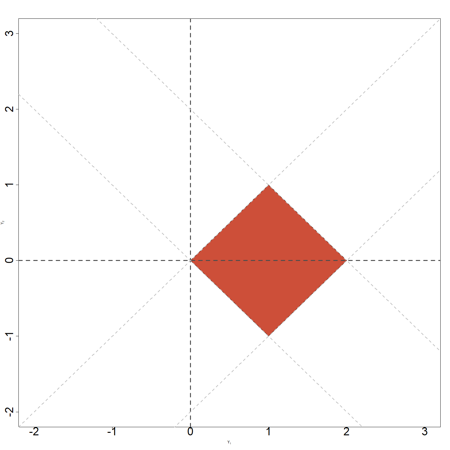
The range of \((Y_1, Y_2)\)
The Jacobian
- With \(X_1 = (Y_1 + Y_2)/2\), \(X_2 = (Y_1 - Y_2)/2\), we find that the Jacobian is given by \[ \begin{aligned} J\left( y \right) &= \det \left( \begin{array}{ccc} \frac{\partial x_{1}}{\partial y_{1}} & & \frac{\partial x_{1}}{\partial y_{2}} \\ & & \\ \frac{\partial x_{2}}{\partial y_{1}} & & \frac{\partial x_{2}}{\partial y_{2}} \end{array} \right) = \det \left( \begin{array}{cc} 1/2 & 1/2 \\ 1/2 & -1/2 \end{array} \right) \\ & \\ &= -1/2 , \end{aligned} \] and the pdf of \((Y_1, Y_2)\) is: \[ f(y_1, y_2) = 1/2 \qquad 0 \le y_1 + y_2 \le 2 \, , \quad 0 \le y_1 - y_2 \le 2 \] (the red polygon).
The marginal of \(Y_1\)
Recall that \[f_{Y_1}(y_1) \, = \, \int f_Y(y_1, y_2) \, dy_2\]
We need to determine the limits of that integral
We know that \(0 \le y_1 \le 2\) and
If \(0 \le y_1 \le 1\) then \(-y_1 \le y_2 \le y_1\)
If \(1 \le y_1 \le 2\) then \(y_1 - 2 \le y_2 \le 2 - y_1\)
The marginal of \(Y_1\)
Hence, if \(0 \le y_1 \le 1\) we have \[f_{Y_1}(y_1) \, = \, \int_{-y_1}^{y_1} (1/2) \, dy_2 = y_1\]
If \(1 \le y_1 \le 2\): \[f_{Y_1}(y_1) \, = \, \int_{y_1-2}^{2-y_1} (1/2) \, dy_2 = 2 - y_1\]
In other words \[f_{Y_1}(y_1) \, = \, \left\{ \begin{array}{ll} y_1 & \mbox{ if } 0 \le y_1 \le 1 \\ 2 - y_1 & \mbox{ if } 1 \le y_1 \le 2 \\ 0 & \mbox{otherwise} \end{array} \right.\]
A good exercise
Repeat this example but using \[ \begin{aligned} \left( \begin{array}{c} Y_{1} \\ \\ Y_{2} \end{array} \right) &= \left( \begin{array}{c} X_{1} + X_{2} \\ \\ X_{2} \end{array} \right) \begin{array}{l} \leftarrow \text{ function of interest } \\ \\ \leftarrow \text{ auxiliary function } \end{array} & \\ \end{aligned} \]
You should obtain the same pdf for \(Y_1\) as before
AND it is much easier!
Example - Polar coordinates
Let \(X_1\) and \(X_2\) be independent standard normal random variables with pdf \[\begin{aligned} f (x_{1},x_{2}) &=& \frac{1}{2\pi }\exp \left ( - (x_{1}^{2}+x_{2}^{2} )/2 \right ) \, , \quad x_1, x_2 \in \mathbb{R}^2.\end{aligned}\]
Work out the joint pdf of \((R, \theta)^\mathsf{T}\): \[\begin{aligned} R &=& \sqrt{X_{1}^{2}+X_{2}^{2}} \\ \theta &=& \arctan ( {X_{2}}/{X_{1}} ) \end{aligned}\]
\((R, \theta) \in [0, +\infty) \times [0, 2\pi)\) are the polar coordinates of \(( X_{1},X_{2}) \in \mathbb{R}^2\).
Remark: one has to interpret \(\arctan(\cdot)\) in a specific way here.
Example - Polar coordinates
The inverse transformation is found to be: \[\begin{aligned} X_{1} &=&R\cos ( \theta ), \\ %&& \\ X_{2} &=&R\sin ( \theta ). \\\end{aligned}\]
The Jacobian is: \[ \begin{aligned} J &= \left\vert \det \left( \begin{array}{cc} \frac{\partial x_{1}}{\partial R} & \frac{\partial x_{1}}{\partial \theta} \\ \frac{\partial x_{2}}{\partial R} & \frac{\partial x_{2}}{\partial \theta} \end{array} \right) \right\vert \\ & \\ &= \left\vert \det \left( \begin{array}{cc} \cos \left( \theta \right) & -R \, \sin \left( \theta \right) \\ \sin \left( \theta \right) & R \, \cos \left( \theta \right) \end{array} \right) \right\vert \\ & \\ &= R \, \cos^{2}\left( \theta \right) + R \, \sin^{2}\left( \theta \right) = R \end{aligned} \]
Example - Polar coordinates
Thus, the (joint) pdf of \(( R,\theta )\) is \[f ( r,\theta ) = \frac{1}{2\pi }r \exp( -r^2 / 2 ) \, \qquad r \ge 0 \, , \quad 0 \le \theta < 2 \, \pi\]
Check that:
\(R\) and \(\theta\) are independent,
\(\theta \thicksim \mathcal{U}(0, 2\pi)\), and
the pdf of \(R\) is: \(f (r) = r \exp( -r^2 / 2 )\) for \(r \geq 0\), known as the Rayleigh distribution.
Stat 302 - Winter 2025/26