Lecture 7: LASSO Regression

Learning Objectives

By the end of this lecture, you should be able to:

1. Implement LASSO regression using both constrained and penalized formulations
2. Identify norm penalties that enforce sparsity versus shrinkage in parameter space
3. Compare and contrast ridge regression vs LASSO in terms of variable selection and shrinkage
4. Reason about when LASSO, ridge, or variants are the most appropriate for a given problem
5. Construct a model selection procedure to choose between LASSO versus ridge

Recap: Ridge Regression, Shrinkage versus Variable Selection

So far we have discussed two modelling choices to reduce variance in linear regression:

1. Variable selection: use a subset of the features (e.g., best subset selection, forward stepwise selection, LAR)
2. Ridge regularization: apply a \(\lambda \Vert \beta \Vert_2^2\) penalty to the optimization objective to shrink coefficients towards zero
3. (There’s always the option of adding more training data.)

• It’s important to note that ridge and variable selection are doing VERY different things!
• Ridge regression shrinks coefficients towards zero, but does not set any coefficients exactly to zero.
• Variable selection methods (best subset, forward stepwise, LAR) set some coefficients exactly to zero, but do not shrink the non-zero coefficients.

Goal: Automatic Variable Selection?

• Ridge added a constraint to our OLS optimization problem to limit the size of the coefficients.

• Maybe we could add a similar constraint to limit the number of non-zero coefficients?

• (Note that having \(< p\) non-zero coefficients, or having \(> 0\) coefficients set to zero, is equivalent to removing some covariates from the model.)

• Such a constraint would yield the following optimization problem:

  \[ \mathrm{argmin}_{\hat \beta} \frac 1 n \sum_{i=1}^n (y_i - x_i^T \hat\beta)^2 \quad \text{subject to } \Vert \hat\beta \Vert_0 < s\]

  where \(\Vert \hat\beta \Vert_0\) is the number of non-zero entries in \(\hat\beta\).

• Unfortunately, this optimization problem takes \(O(2^p)\) time to solve.

  Why?

  • Mathematically, it is a NP-hard optimization problem.
  • Intuitively, solving this problem is equivalent to exhaustive subset search that you probably learned about in STAT 306. There are \(2^p\) possible subsets of \(p\) features, and we would need to evaluate the training error for each subset to find the best one.

• Fortunately, we can solve a simpler optimization problem that encourages sparsity in the coefficients. (Mathematically, we solve a convex relaxation).

Solution: Diamond Constraint Regions

• Recall that ridge constrained our solutions so that the \(\beta\) vector lied within a circle (or sphere, or hypersphere) of radius \(s\).
• Instead, what if we set our constraint region to be a diamond?

Illustration of the diamond constraint region for linear regression. It’s likely that, for a “tight-enough” diamond constraint, the minimal solution in the constraint region will live in one of the corners of the diamond, which corresponds to zero-ing out one or more coefficients.

• The minimum sum-of-squares solution under this constraint will (not always, but often) be at a corner of the diamond, which is where one or more coefficients are exactly zero.

• Crucially, the sum-of-squares objective with this diamond constraint is a convex optimization problem that can be solved efficiently!

LASSO Regression

• LASSO regression aims to (approximately) do automated variable selection using this diamond constraint.
• It is another regularized regression method, like ridge regression, which will reduce variance (at the expense of a bit of bias).
• Unlike ridge regression, the constraint/regularization yields a different effect on the learned coefficients: it encourages sparsity (i.e. some coefficients exactly zero) rather than just shrinkage (i.e. all coefficients small but non-zero).

Constrained Formulation

• This diamond constraint region is mathematically defined by the set of all \(\hat \beta\) where

  \[ \Vert \hat\beta \Vert_1 := \sum_{j=1}^p |\hat\beta_j| < s\]

  which yields the constrained optimization problem

  \[ \mathrm{argmin}_{\hat \beta} \frac 1 n \sum_{i=1}^n (y_i - x_i^T \hat\beta)^2 \quad \text{subject to } \Vert \hat\beta \Vert_1 < s\]

• Compare this to the ridge regression constrained optimization problem. For ridge, the constraint was \(\Vert \hat\beta \Vert_2^2 < s\) (i.e. a circle/sphere/hypersphere constraint rather than a diamond). Otherwise the problems are identical.

Regularized (Penalized) Formulation

• As with ridge regression, we can rewrite the constrained optimization problem as a penalized optimization problem:

  \[ \mathrm{argmin}_{\hat \beta} \frac 1 n \sum_{i=1}^n (y_i - x_i^T \hat\beta)^2 + \lambda \Vert \hat\beta \Vert_1 \]

  where again each value of \(s\) in our constrained formulation corresponds to a value of \(\lambda\) in our penalized formulation.

Computing the LASSO Estimator

• Unlike ridge regression, there is no closed-form solution for the LASSO estimator \(\hat\beta_\lambda\).
• Instead, we must use numerical optimization to solve the penalized optimization problem.

TipHow do we Numerically Optimize the LASSO Objective?

(Advanced content for those who are interested)

• The LASSO problem is a convex optimization problem, so typically optimizers like gradient descent will (in theory) converge to the global optimum.
• However, gradient descent doesn’t do well with the non-differentiable corners of the \(\ell_1\) norm.
• Instead, it’s common to use coordinate descent (which is what glmnet uses).
• Proximal gradient descent algorithms are also popular for solving the LASSO problem.

Aside: Regularization with Other Vector Norms

• The ridge regularization penalty (\(\Vert \beta \Vert_2^2\)), the LASSO regularization penalty (\(\Vert \beta \Vert_1\)), and the “sparsity” penalty (\(\Vert \beta \Vert_0\)) are all examples of vector norm penalties.

• More specifically, each is an example of a \(\ell_p\)-norm, where the general form is given by:

  \[\Vert \beta \Vert_p = \left( \sum_{j=1}^p |\beta_j|^p \right)^{1/p}\]

• Below is a plot of values of the constraint \(\Vert \beta \Vert_p = 1\) for various values of \(p\):

• Any of these norms could be used as a regularization penalty in linear regression (though some may yield hard-to-solve optimization problems).

library(mvtnorm)
library(tidyverse)
normBall <- function(q = 1, len = 1000) {
  tg <- seq(0, 2 * pi, length = len)
  out <- data.frame(x = cos(tg)) |>
    mutate(b = (1 - abs(x)^q)^(1 / q), bm = -b) |>
    gather(key = "lab", value = "y", -x)
  out$lab <- paste0('"||" * beta * "||"', "[", signif(q, 2), "]")
  return(out)
}

ellipseData <- function(n = 100, xlim = c(-2, 3), ylim = c(-2, 3),
                        mean = c(1, 1), Sigma = matrix(c(1, 0, 0, .5), 2)) {
  df <- expand.grid(
    x = seq(xlim[1], xlim[2], length.out = n),
    y = seq(ylim[1], ylim[2], length.out = n)
  )
  df$z <- dmvnorm(df, mean, Sigma)
  df
}

lballmax <- function(ed, q = 1, tol = 1e-6) {
  ed <- filter(ed, x > 0, y > 0)
  for (i in 1:20) {
    ff <- abs((ed$x^q + ed$y^q)^(1 / q) - 1) < tol
    if (sum(ff) > 0) break
    tol <- 2 * tol
  }
  best <- ed[ff, ]
  best[which.max(best$z), ]
}

nbs <- list()
nbs[[1]] <- normBall(0, 1)
qs <- c(.5, 1, 1.5, 2, 20)
for (ii in 2:6) nbs[[ii]] <- normBall(qs[ii - 1])
nbs[[1]]$lab <- paste0('"||" * beta * "||"', "[0.0]")
nbs[[4]]$lab <- paste0('"||" * beta * "||"', "[1.0]")
nbs <- bind_rows(nbs)
nbs$lab <- factor(nbs$lab, levels = unique(nbs$lab))
seg <- data.frame(
  lab = levels(nbs$lab)[1],
  x0 = c(-1, 0), x1 = c(1, 0), y0 = c(0, -1), y1 = c(0, 1)
)
levels(seg$lab) <- levels(nbs$lab)
ggplot(nbs, aes(x, y)) +
  geom_path(size = 1.2) +
  facet_grid(.~lab, labeller = label_parsed) +
  geom_segment(data = seg, aes(x = x0, xend = x1, y = y0, yend = y1), size = 1.2) +
  theme_bw(base_family = "", base_size = 24) +
  coord_equal() +
  scale_x_continuous(breaks = c(-1, 0, 1)) +
  scale_y_continuous(breaks = c(-1, 0, 1)) +
  geom_vline(xintercept = 0, size = .5) +
  geom_hline(yintercept = 0, size = .5) +
  xlab(bquote(beta[1])) +
  ylab(bquote(beta[2]))

Important Special Cases

• \(p = 0\) is the number of non-zero entries in \(\beta\) (the “sparsity” penalty)
• \(p = \infty\) is the maximum absolute value of any entry in \(\beta\) (the “max” penalty)
• \(p \geq 1\) gives a convex function of \(\beta\), which makes optimization nice
• \(p < 2\) gives a norm with “corners” (i.e., non-differentiable points on the axes), which encourage sparsity

Example: LASSO versus Ridge Regression

• Here we’re going to run both ridge and LASSO regression on the prostate cancer dataset from Lab 01.
• I will do a CV sweep to find the best regularization parameter \(\lambda\) for each method.
• Again we’ll use glmnet to fit both models.
  • The argument alpha = 1 in cv.glmnet specifies LASSO, while alpha = 0 specifies ridge regression.

library(glmnet)
data(prostate, package = "ElemStatLearn")
X <- prostate |> dplyr::select(-train, -lpsa) |>  as.matrix()
Y <- prostate$lpsa
lasso <- cv.glmnet(x = X, y = Y) # alpha = 1 by default
ridge <- cv.glmnet(x = X, y = Y, alpha = 0)

• Now let’s plot the CV curves and coefficient paths for both ridge and LASSO as functions of their regularization parameter \(\lambda\).
• Note that we cannot compare the \(\lambda\) values directly between ridge and LASSO, since they are on different scales.
• (The \(\lambda\) values also don’t have any intrinsic meaning. Larger values imply more regularization, but a \(\lambda = 4.7\) means nothing in isolation.)

par(mfrow = c(2, 2))
# Get y-axis range for consistent scaling
ridge_mse <- range(c(ridge$cvm - ridge$cvsd, ridge$cvm + ridge$cvsd))
lasso_mse <- range(c(lasso$cvm - lasso$cvsd, lasso$cvm + lasso$cvsd))
ylim_range <- range(ridge_mse, lasso_mse)
plot(ridge, main = "Ridge CV", ylim = ylim_range)
plot(lasso, main = "LASSO CV", ylim = ylim_range)

# Get coefficient range for consistent scaling
ridge_coef_range <- range(ridge$glmnet.fit$beta)
lasso_coef_range <- range(lasso$glmnet.fit$beta)
coef_ylim <- range(ridge_coef_range, lasso_coef_range)
plot(ridge$glmnet.fit, main = "Ridge Coeffs.", xvar = "lambda", ylim = coef_ylim)
abline(h = 0, lty = 2)
plot(lasso$glmnet.fit, main = "LASSO Coeffs.", xvar = "lambda", ylim = coef_ylim)
abline(h = 0, lty = 2)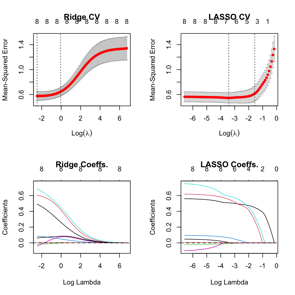

• The numbers on the top of the plots indicate the number of non-zero coefficients at each value of \(\lambda\).
• Notice that ridge regression always has all 8 coefficients non-zero, while LASSO sets some coefficients exactly to zero for larger values of \(\lambda\).

When Should I Consider using Ridge over LASSO?

1. If all of the covariates are truly relevant, and dropping too many of them would hurt accuracy

   Why?

   • LASSO tends to select only a few variables, and set the rest to zero. If all variables are relevant, this can lead to underfitting.
   • Ridge regression, on the other hand, shrinks all coefficients towards zero, but keeps them all in the model.

2. If I create a one-hot encoding of a categorical variable with many levels (e.g., ZIP code)

   Why?

   • LASSO might drop some of the levels but not others, which can be hard to interpret
   • Ridge regression will tend to keep all levels, but shrink them towards zero
   • A variant of LASSO called the group LASSO can be used to select or drop all levels of a categorical variable together.

3. If computational resources are limited

   Why?

   • LASSO requires numerical optimization to solve, while ridge regression has a closed-form solution.
   • We have to run multiple optimization problems for each value of \(\lambda\) we want to test in cross-validation.
   • Ridge regression only requires a single SVD, which can be reused for all values of \(\lambda\).
   • Moreover, as we will see in a later lecture, we can compute the LOO-CV risk estimate for ridge almost for free, while LASSO requires refitting the model \(n\) times.

CautionWhen Should I Avoid Using Both Ridge and LASSO?

If I’m in a high-bias/low-variance regime to begin with, I shouldn’t use either method.

Why?

• Regularization (both ridge and LASSO) increases bias but reduces variance.
• If the un-regularized model is already low variance, regularization will likely hurt performance.

Important Practical Considerations when Using LASSO or Ridge Regression

1. The intercept \(\hat \beta_0\) is never penalized!

   Why?

   • The intercept parameter is an estimate of the mean of \(Y\), and we generally do not want to shrink this estimate.
   • In practice, we usually standardize the response to have mean zero and variance one before fitting a regularized regression model.

2. It’s important to center the features (i.e. subtract off each covariate’s empirical mean) before fitting.

   Why?

   • If the features are not centered, the intercept will implicitly be penalized, which can lead to suboptimal performance.
   • Centering the features ensures that the intercept is the mean of \(Y\) when all other covariates are zero.
   • Standardizing the features (i.e. scaling them to have unit variance) is also common, but not strictly necessary for LASSO or ridge regression.

3. Categorical parameters require special care with LASSO.

   Why?

   • See above

4. Ridge or LASSO penalties can be used in other (non-linear regression) models.

Summary

• Ridge regression applies an \(\ell_2\) penalty to shrink coefficients towards zero, but does not set any coefficients exactly to zero.
• LASSO regression applies an \(\ell_1\) penalty to encourage sparsity in the coefficients, setting some coefficients exactly to zero.
• LASSO requires numerical optimization to solve, and care is needed when using categorical variables.
• Both ridge and LASSO increase bias but reduce variance.
• The choice between ridge and LASSO depends on the specific problem and goals of the analysis.