Lecture 8: Basis Expansions

Learning Objectives

By the end of this lecture, you should be able to:

1. Construct polynomial, spline, and Fourier basis expansions for regression
2. Select appropriate basis functions based on problem characteristics
3. Articulate how basis expansions affect bias and variance
4. Differentiate between linearity and nonlinearity in terms of parameterization versus functional form

Overview

We have spent the last few lectures discussing methods to reduce variance in linear models.

0. Manual variable selection
1. Ridge regression (shrink all parameters)
2. Lasso regression (set some parameters to zero)

• In this lecture, we will focus on the other side of the bias-variance tradeoff, and introduce a method to reduce bias in linear models.
• Crucially, our bias reduction method will allow us to retain linearity with respect to the learned parameters while allowing for nonlinearity with respect to the input features.
• The method, basis expansions, is a generalization of the idea of interaction terms that you saw in STAT 306.

Motivation

• We have typically assumed a statistical model where \(\mathbb E[Y \mid X]\) is a linear function of the input features \(X\), i.e. \(\mathbb E[Y \mid X] = X^\top \beta\) for some \(\beta \in \mathbb R^p\).

• We will now relax this assumption of linearity, and instead assume that

  \[\mathbb E[Y \mid X] = f(X)\]

  for some unknown function \(f: \mathbb R^p \to \mathbb R\).

• Using a predictive model of the form \(\hat f_\mathcal{D}(X) = X^\top \hat \beta\), like what we get from OLS, will not work well if \(f\) is highly nonlinear; it will be a high-bias predictor.

ImportantBut Isn’t OLS Unbiased?

• Recall that OLS is unbiased only under the assumptions made by the linear statistical model.
• Under the more general model \(\mathbb E[Y \mid X] = f(X)\), OLS is biased unless \(f\) is actually linear.
• To see why this is the case, let’s do a Taylor expansion of \(f\) around \(0\).

\[f(X) = f(0) + \nabla f(0)^\top X + \frac{1}{2} X^\top H_f(0) X + \ldots\]

Even if OLS were to perfectly estimate \(\hat \beta = \nabla f(0)\), the higher-order terms would still be missing, and so \(\mathbb E[\hat f_\mathcal{D}(X) \mid X] \neq f(X)\).

TipQuiz: Will Ridge or Lasso Be Beneficial in this Situation?

Probably not.

• Ridge and Lasso reduce variance and introduce bias, and we will likely be in a high-bias situation already.
• More specifically, Ridge and Lasso still produce predictors of the form \(\hat f_\mathcal{D}(X) = X^\top \hat \beta\), which are still missing the higher-order terms that create the bias problem in the first place.

Warmup: Polynomial Basis Expansions for \(p=1\)

• Why don’t we just use a predictive model that includes the higher-order terms?

• For example, if \(p=1\), we could learn a model of the form:

  \[\hat f_\mathcal{D}(x) = \hat \beta_0 + \hat \beta_1 x + \hat \beta_2 x^2 + \ldots + \hat \beta_d x^d.\]

• As \(d \to \infty\), there exists some set of coefficients \(\hat \beta_0, \ldots, \hat \beta_d\) such that \(f(x) = \sum_{j=0}^d \beta_j x^j\).

• This model is known as a polynomial regression model, or a polynomial basis expansion.

NoteLinearity vs. Nonlinearity

• This model is non-linear in \(X\) (because of the \(x^2, \ldots, x^d\) terms)
• However, it is still linear in the parameters \(\hat \beta_0, \ldots, \hat \beta_d\).
• Therefore, we can pretend as if we have a dataset with \(d\) features \((X, X^2, \ldots, X^d)\) and use OLS/Ridge/LASSO to learn the parameters \(\hat \beta_0, \ldots, \hat \beta_d\).

Bias Reduction

Using higher-order polynomial terms can significantly reduce bias.

• Let’s assume that, under our statistical model, \(\mathbb E[Y \mid X] = f(x)\) for some \(d^\mathrm{th}\) degree polynomial \(f\).

• Let’s also assume that we use a \(d^\mathrm{th}\) degree polynomial basis expansion to learn a predictor \(\hat f_\mathcal{D}(x) = \sum_{j=0}^d \hat \beta_j x^j\) using OLS.

• Then \(\hat f_\mathcal{D}(x)\) is an unbiased estimator of \(f(x)\)!

  Why

  • Again, we can pretend as if we’re working with a dataset with \(d\) features \((X, X^2, \ldots, X^d)\).
  • Under our statistical model, \(\mathbb E[Y \mid X, X^2, \ldots, X^d] = \sum_{i=1}^d \beta_i X^i\)
  • By what we derived two lectures ago, OLS with the features \((X, X^2, \ldots, X^d)\) will be unbiased for estimating \(\beta_0, \ldots, \beta_d\).

Example

• Below we’ll plot the OLS fit using polynomial basis expansions of different orders on the arcuate dataset from the Stat406 package.
• The standard linear model (no basis expansion) is a poor fit for the data. This error is likely due to high bias, because there’s enough data to estimate two parameters with little variance, but the linear model is too simple to capture the relationship between position and fa.
• As we increase the order of the polynomial basis expansion, the fit improves significantly, and the bias is reduced.

set.seed(406406)
library(tidyverse)
data(arcuate, package = "Stat406")
arcuate <- arcuate |> slice_sample(n = 220)
arcuate |>
  ggplot(aes(position, fa)) +
  geom_point(color = "black") +
  geom_smooth(aes(color = "a"), formula = y ~ x, method = "lm", se = FALSE) +
  geom_smooth(aes(color = "b"), formula = y ~ poly(x, 4), method = "lm", se = FALSE) +
  geom_smooth(aes(color = "c"), formula = y ~ poly(x, 7), method = "lm", se = FALSE) +
  geom_smooth(aes(color = "d"), formula = y ~ poly(x, 25), method = "lm", se = FALSE) +
  scale_color_manual(
    name = "Taylor order",
    values = c("a" = "grey", "b" = "blue", "c" = "red", "d" = "green"),
    labels = c("1 term", "4 terms", "7 terms", "25 terms")
  )

Polynomial Basis Expansions for \(p>1\)

• For \(p>1\), we have to include a few more terms.

• For \(x \in \mathbb R^p\), the Taylor expansion of \(f(x)\) around \(0\) is:

  \[f(X) = f(0) + \nabla f(0)^\top X + \frac{1}{2} X^\top H_f(0) X + \ldots,\]

  where \(\nabla f(0) \in \mathbb R^p\) is the gradient of \(f\) at \(0\), and \(H_f(0) \in \mathbb R^{p \times p}\) is the Hessian of \(f\) at \(0\).

• The gradient has \(p\) entries, and the Hessian has \(p(p+1)/2\) unique entries (since it is a symmetric matrix).

• Thus, the second-order polynomial basis expansion will be of the form:

  \[\hat f_\mathcal{D}(x) = \hat \beta_0 + \sum_{j=1}^p \hat \beta_j x_j + \sum_{j=1}^p \sum_{k=j}^p \hat \beta_{jk} x_j x_k.\]

• The \(\beta_{jk}\) parameters for \(j \neq k\) are called interaction terms, which you studied in STAT 306.

• This model contains \(1 + p + p(p+1)/2 = 1 + p(p+3)/2\) parameters, which is \(O(p^2)\).

• If \(n\) is not much larger than \(p^2\), then including these interaction terms could push us back into a high-variance regime.

• We will come back to this parameter growth issue in the next module.

TipBasis Expansions and Regularization

• If \(p\) is large, it may be a good idea to use basis expansions in conjunction with Ridge or Lasso.
• Adding \(O(p^2)\) interaction terms will reduce bias (at the cost of increased variance), and Ridge/Lasso can help reduce the variance that is introduced.
• This is just one example where we need to use both bias reduction and variance reduction techniques together to get a good predictor!

Other Basis Expansions

• Besides polynomials, there are two other common basis expansions: Fourier basis expansions and splines.
• As with polynomials, both create nonlinear functions of the input features while remaining linear in the parameters.

Fourier Basis Expansions

• Recall that (most) \(\mathbb R \to \mathbb R\) functions can be expressed by their Fourier series:

  \[f(x) = a_0 + \sum_{j=1}^\infty a_j \cos(j 2 \pi x) + b_j \sin(j 2 \pi x)\]

• We can thus consider a predictive model of the form:

  \[\hat f_\mathcal{D}(x) = \hat a_0 + \sum_{j=1}^d \hat a_j \cos(j 2 \pi x) + \hat b_j \sin(j 2 \pi x)\]

  for some \(d \in \mathbb N\).

• Higher values of \(d\) will be capable of fitting more complex functions (i.e. reduce bias), but as \(d\) gets close to \(n\), we will likely enter a high-variance regime.

Splines

• A spline is a piecewise polynomial function that is smooth at the places where the pieces meet.

• For example, a linear spline is a function of the form:

  \[ f(x) = \begin{cases} \beta_0 + \beta_1 x & x < k_1 \\ \beta_0 + \beta_1 x + \beta_2 (x - k_1) & k_1 \leq x < k_2 \\ \beta_0 + \beta_1 x + \beta_2 (x - k_1) + \beta_3 (x - k_2) & k_2 \leq x < k_3 \\ \ldots \end{cases} \]

  where \(k_1, k_2, \ldots\) are called knots.

• The function is continuous at the knots, but not differentiable.

• Again, increasing the number of knots will reduce bias but increase variance.

Comparison of Basis Expansions

• Below is a comparison of the first 5 “features” created by each of the three basis expansions we discussed: polynomial, linear splines, and Fourier for a \(p=1\) input.
• All three basis expansions can represent (nearly) all functions as \(d\to\infty\), but some basis expansions may be more appropriate for certain problems for a fixed value of \(d\).

library(cowplot)
library(ggplot2)

relu_shifted <- function(x, shift) {pmax(0, x - shift)}

# Create a sequence of x values
x_vals <- seq(-3, 3, length.out = 1000)

# Create a data frame with all the shifted functions
data <- data.frame(
  x = rep(x_vals, 5),
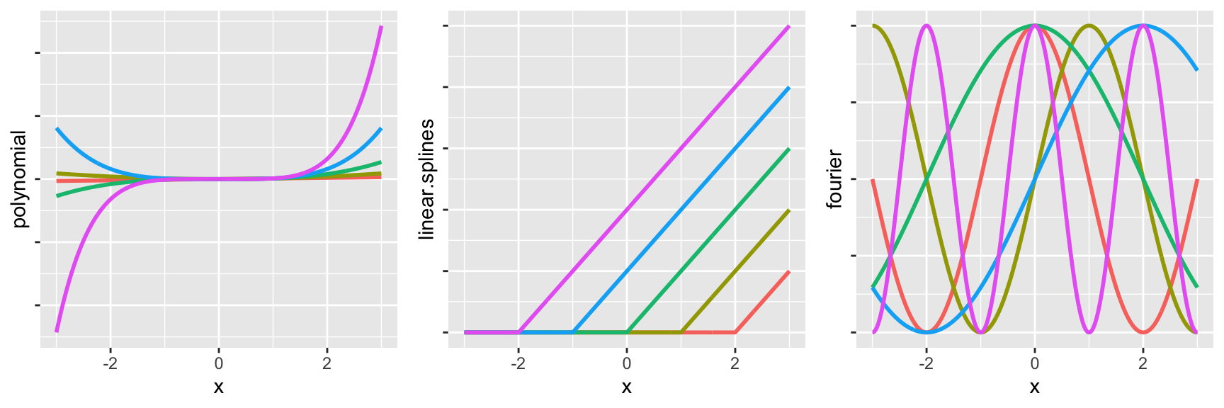
  polynomial = c(x_vals, x_vals^2, x_vals^3, x_vals^4, x_vals^5),
  linear.splines = c(relu_shifted(x_vals, 2), relu_shifted(x_vals, 1), relu_shifted(x_vals, 0), relu_shifted(x_vals, -1), relu_shifted(x_vals, -2)),
  fourier = c(cos(pi / 2 * x_vals), sin(pi / 2 * x_vals), cos(pi / 4 * x_vals), sin(pi / 4 * x_vals), cos(pi * x_vals)),
  function_label = rep(c("f1", "f2", "f3", "f4", "f5"), each = length(x_vals))
)

# Plot using ggplot2
g1 <- ggplot(data, aes(x = x, y = polynomial, color = function_label)) +
      geom_line(size = 1, show.legend=FALSE) +
      theme(axis.text.y=element_blank())
g2 <- ggplot(data, aes(x = x, y = linear.splines, color = function_label)) +
      geom_line(size = 1, show.legend=FALSE) +
      theme(axis.text.y=element_blank())
g3 <- ggplot(data, aes(x = x, y = fourier, color = function_label)) +
      geom_line(size = 1, show.legend=FALSE) +
      theme(axis.text.y=element_blank())

plot_grid(g1, g2, g3, ncol = 3)

NoteChoosing a Basis Expansion

• There is no universally best basis expansion.
• You can try all three basis expansions and use cross-validation to select the best one.
• You can include combinations of basis expansions (e.g. polynomial + splines), and use LASSO to select the best ones.
• You can also use domain knowledge to select a basis expansion that is appropriate for your problem.

Summary

• Basis expansions are a method to reduce bias in linear models by allowing for nonlinearity with respect to the input features while retaining linearity with respect to the parameters.
• Common basis expansions include polynomial basis expansions, Fourier basis expansions, and splines.
• Basis expansions can be used in conjunction with Ridge or Lasso to control variance when the number of parameters grows large.
• There is no universally best basis expansion; you can try multiple basis expansions.
• The number of parameters for basis expansions can grow quickly with the number of input features; we will discuss this issue in more detail in the next module.