Can we find a parametric model that approximates kNN?
What Does a kNN Function Look Like?
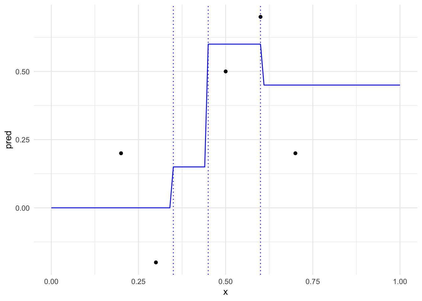
kNN regression produces a piecewise constant function.
Consider the subset of all points \(S \subset \mathcal X\) that each have \(X_{i1}, \ldots, X_{ij}\) as their \(k\) nearest neighbors.
For all \(x \in S\), the kNN regression function is constant: \[
\hat{f}_{\mathrm{kNN}}(x) = \frac{1}{k} \sum_{X_i \in N_k(x)} Y_i = \text{constant for all } x \in S.
\]
More generally, given all subsets \(S_1, \ldots, S_m\) of \(\mathcal X\) where each point in \(S_j\) has the same \(k\) nearest neighbors, the kNN regression function is piecewise constant over these subsets.
The subsets \(S_1, \ldots, S_m\) are referred to as Voronoi cells, and they are convex polytopes in \(\mathbb{R}^p\).
Let’s assume we want to build a piecewise constant predictive model. kNN gives us one way to do this, but is there a parametric model that achieves something similar?
Since kNN is non-parametric, we define the piecewise constant regions (i.e. the Voronoi cells \(S_1, \ldots, S_m\)) implicitly through the training data.
What if we instead defined the piecewise constant regions by explicitly defining the boundaries of the regions?
To simplify, let’s assume that the piecewise constant regions are axis-aligned rectangles in \(\mathbb{R}^p\).
While there are many mechanisms for representing such piecewise constant functions, one of the most common is through decision trees.
Decision Trees for Regression and Classification
A decision tree is a learned binary tree structure that recursively partitions the predictor space into axis-aligned rectangles.
Each of the leaf nodes of the tree corresponds to a single rectangle in the predictor space.
Each internal node of the tree corresponds to a decision rule that recursively splits the predictor space along one of the covariate dimensions.
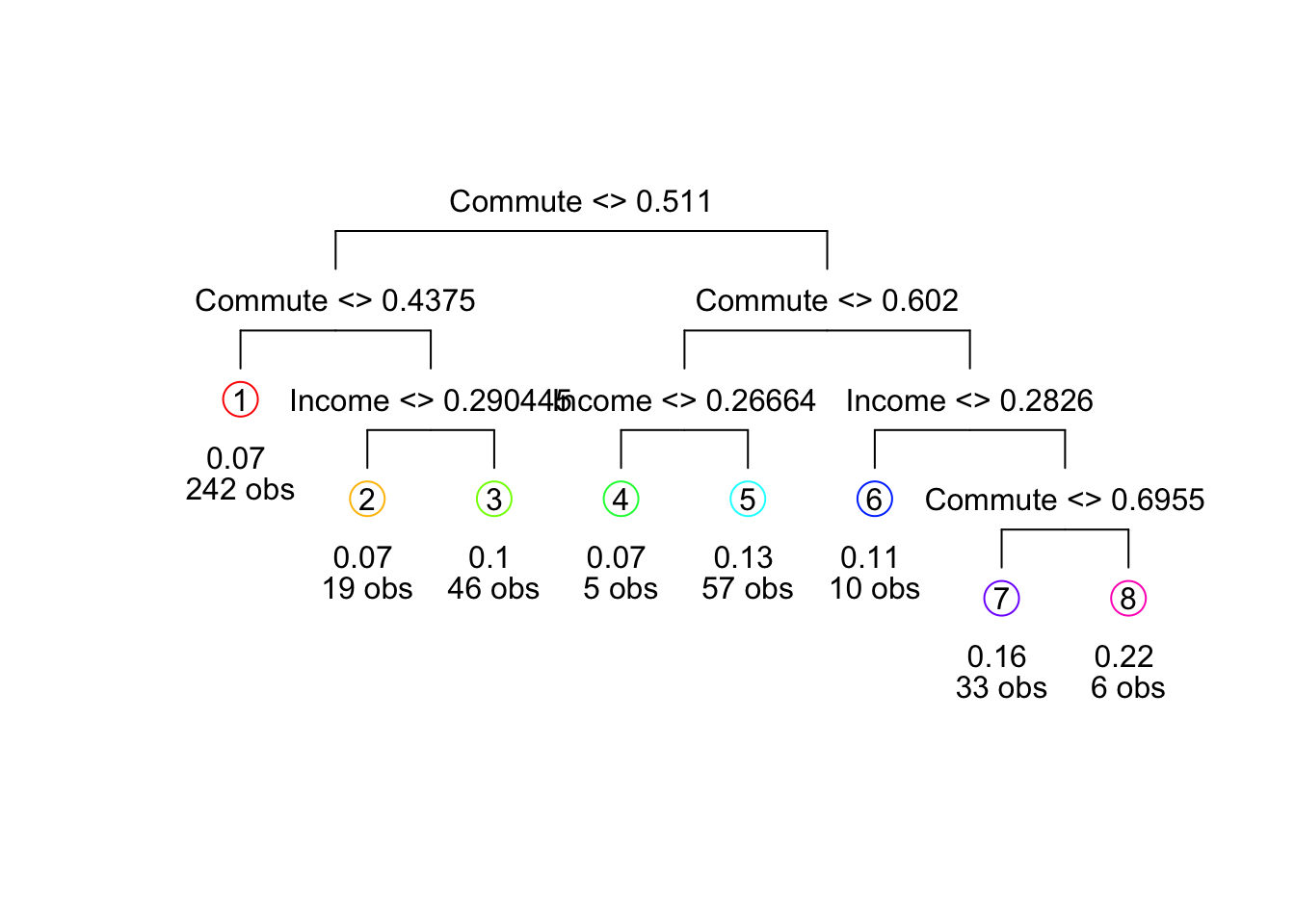
A Simple Example
Consider the decision tree above for a regression problem with two predictors, \(X_1 = \mathrm{Commute}\) and \(X_2 = \mathrm{Income}\) to predict \(Y = \mathrm{Mobility}\).
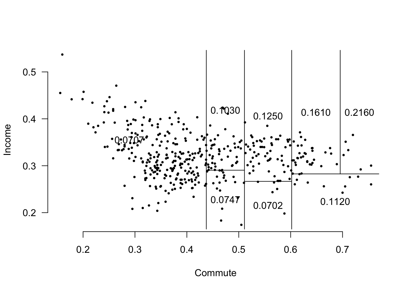
The splits result in the following piecewise constant regions in the prediction space:
The axis-aligned rectangles are “simpler shapes” than the Voronoi cells, which can be more complex polytopes, and so kNN can approximate more complex functions than a decision tree of similar complexity.
Additionally, the number of piecewise constant regions created by kNN is combinatorial in \(n\) and \(p\), while the number of piecewise constant regions created by a decision tree is linear in the number of splits.
However, the nonparametric nature of kNN requires storing all training data, while a decision tree only requires storing the tree structure and the values at the leaf nodes.
Moreover, limiting the piecewise constant regions to axis-aligned rectangles also reduces the effects of the curse of dimensionality (though decision trees by themselves are usually either high-bias or high-variance models, as we will see later).
Tree Depth, Bias, and Variance
The depth of a decision tree is the length of the longest path from the root node to any leaf node.
Typically, we control the complexity of a decision tree by limiting its depth.
If \(\mathrm{depth} = \infty\), then the leaf nodes of the decision tree will correspond to single training examples.
TipQuiz: Effect of Depth
A deeper decision tree will generally have (lower/higher) bias and (lower/higher) variance, while a shallower decision tree will generally have (lower/higher) bias and (lower/higher) variance.
Answer
A deeper decision tree will generally have lower bias and higher variance, while a shallower decision tree will generally have higher bias and lower variance.
A very deep tree will have one piecewise constant region per training example. Such a predictor will be highly dependent on the particular training sample, resulting in high variance.
A very shallow tree will only have a few piecewise constant regions. On any training sample, the resulting model will be too simple to capture the underlying structure of the data, resulting in high bias.
Learning a Decision Tree from Data
Given a fixed depth \(d\), how do we learn a decision tree from data? We formulate the learning problem as an optimization problem over training data!
What makes a good tree? If a piecewise constant function is going to approximate our data well, then we want all responses within a given piece to be as similar as possible. In other words, we want to minimize the impurity of each leaf node.
Minimizing the impurity of all depth-\(d\) trees is a NP-hard problem, so instead we use a greedy strategy.
We will iteratively construct a depth-\(d\) tree, taking the most “impure” leaf node at each step and splitting it to reduce its impurity as much as possible.
Metrics of Impurity
Regression problems: we want to minimize the variance of responses within each piecewise region: \(\widehat{\mathrm{Var}} = \frac{1}{n-1} \sum_{i=1}^n (Y_i - \bar{Y})^2\), where \(\bar{Y}\) is the average response of all training points in the leaf.
Classification problems: rather than minimizing variance, it is common to minimize Gini impurity of responses, \(\hat G = \hat p (1 - \hat p)\), where \(\hat p\) is the proportion of training points in the leaf with \(Y=1\).
Introducing a New Split
We will choose to split the most impure leaf node at each step.
We will split this most impure leaf node \(R\) into two child nodes \(R^>\) and \(R^<\).
To do this, we will consider all possible splits along all \(p\) predictor dimensions.
Mathematically:
For a given splitting variable\(j\) and split value\(s\), define \[
\begin{align}
R^> &= \{x \in R : x^{(j)} > s\} \\
R^< &= \{x \in R : x^{(j)} < s\}
\end{align}
\]
When choosing a split for a given leaf node, we want to choose the split that minimizes the weighted impurity of the resulting child nodes.
Advantages and Disadvantages of Decision Trees
🎉 Trees are very easy to explain (much easier than even linear regression).
🎉 Some people believe that decision trees mirror human decision.
🎉 Trees can easily be displayed graphically no matter the dimension of the data.
🎉 Trees can easily handle qualitative predictors without the need to create dummy variables.
💩 Trees aren’t very good at prediction.
💩 Trees are highly variable. Small changes in training data \(\Longrightarrow\) big changes in the tree.
To fix these last two, we can try to grow many trees and average their performance. We will cover this strategy in the next module.
Summary
Decision trees are the parametric counterpart to kNN regression/classification.
Like kNN, decision trees produce piecewise constant predictions.
Unlike kNN, these piecewise constants are not defined through training data and are instead constrained to be axis-aligned rectangles.
The depth of decision trees controls the bias-variance tradeoff, where maximum depth corresponds to piecewise regions that contain only a single training point.
Trees are constructed in a greedy fashion by iteratively splitting the most impure leaf node to reduce its impurity as much as possible.
While decision trees are easy to interpret and explain, they tend to have high variance and/or high bias, leading to poor predictive performance.