15 LDA and QDA

Stat 406

Daniel J. McDonald

Last modified – 09 October 2023

\[ \DeclareMathOperator*{\argmin}{argmin} \DeclareMathOperator*{\argmax}{argmax} \DeclareMathOperator*{\minimize}{minimize} \DeclareMathOperator*{\maximize}{maximize} \DeclareMathOperator*{\find}{find} \DeclareMathOperator{\st}{subject\,\,to} \newcommand{\E}{E} \newcommand{\Expect}[1]{\E\left[ #1 \right]} \newcommand{\Var}[1]{\mathrm{Var}\left[ #1 \right]} \newcommand{\Cov}[2]{\mathrm{Cov}\left[#1,\ #2\right]} \newcommand{\given}{\ \vert\ } \newcommand{\X}{\mathbf{X}} \newcommand{\x}{\mathbf{x}} \newcommand{\y}{\mathbf{y}} \newcommand{\P}{\mathcal{P}} \newcommand{\R}{\mathbb{R}} \newcommand{\norm}[1]{\left\lVert #1 \right\rVert} \newcommand{\snorm}[1]{\lVert #1 \rVert} \newcommand{\tr}[1]{\mbox{tr}(#1)} \newcommand{\brt}{\widehat{\beta}^R_{s}} \newcommand{\brl}{\widehat{\beta}^R_{\lambda}} \newcommand{\bls}{\widehat{\beta}_{ols}} \newcommand{\blt}{\widehat{\beta}^L_{s}} \newcommand{\bll}{\widehat{\beta}^L_{\lambda}} \]

Last time

We showed that with two classes, the Bayes’ classifier is

\[g_*(X) = \begin{cases} 1 & \textrm{ if } \frac{p_1(X)}{p_0(X)} > \frac{1-\pi}{\pi} \\ 0 & \textrm{ otherwise} \end{cases}\]

where \(p_1(X) = Pr(X \given Y=1)\), \(p_0(X) = Pr(X \given Y=0)\) and \(\pi = Pr(Y=1)\)

For more than two classes.

\[g_*(X) = \argmax_k \frac{\pi_k p_k(X)}{\sum_k \pi_k p_k(X)}\]

where \(p_k(X) = Pr(X \given Y=k)\) and \(\pi_k = P(Y=k)\)

Estimating these

Let’s make some assumptions:

1. \(Pr(X\given Y=k) = \mbox{N}(\mu_k,\Sigma_k)\)
2. \(\Sigma_k = \Sigma_{k'} = \Sigma\)

This leads to Linear Discriminant Analysis (LDA), one of the oldest classifiers

LDA

1. Split your training data into \(K\) subsets based on \(y_i=k\).
2. In each subset, estimate the mean of \(X\): \(\widehat\mu_k = \overline{X}_k\)
3. Estimate the pooled variance: \[\widehat\Sigma = \frac{1}{n-K} \sum_{k \in \mathcal{K}} \sum_{i \in k} (x_i - \overline{X}_k) (x_i - \overline{X}_k)^{\top}\]
4. Estimate the class proportion: \(\widehat\pi_k = n_k/n\)

LDA

Assume just \(K = 2\) so \(k \in \{0,\ 1\}\)

We predict \(\widehat{y} = 1\) if

\[\widehat{p_1}(x) / \widehat{p_0}(x) > \widehat{\pi_0} / \widehat{\pi_1}\]

Plug in the density estimates:

\[\widehat{p_k}(x) = N(x - \widehat{\mu}_k,\ \widehat\Sigma)\]

LDA

Now we take \(\log\) and simplify \((K=2)\):

\[ \begin{aligned} &\Rightarrow \log(\widehat{p_1}(x)\times\widehat{\pi_1}) - \log(\widehat{p_0}(x)\times\widehat{\pi_0}) = \cdots = \cdots\\ &= \underbrace{\left(x^\top\widehat\Sigma^{-1}\overline X_1-\frac{1}{2}\overline X_1^\top \widehat\Sigma^{-1}\overline X_1 + \log \widehat\pi_1\right)}_{\delta_1(x)} - \underbrace{\left(x^\top\widehat\Sigma^{-1}\overline X_0-\frac{1}{2}\overline X_0^\top \widehat\Sigma^{-1}\overline X_0 + \log \widehat\pi_0\right)}_{\delta_0(x)}\\ &= \delta_1(x) - \delta_0(x) \end{aligned} \]

If \(\delta_1(x) > \delta_0(x)\), we set \(\widehat g(x)=1\)

One dimensional intuition

set.seed(406406406)
n <- 100
pi <- .6
mu0 <- -1
mu1 <- 2
sigma <- 2
tib <- tibble(
  y = rbinom(n, 1, pi),
  x = rnorm(n, mu0, sigma) * (y == 0) + rnorm(n, mu1, sigma) * (y == 1)
)

Code

gg <- ggplot(tib, aes(x, y)) +
  geom_point(colour = blue) +
  stat_function(fun = ~ 6 * (1 - pi) * dnorm(.x, mu0, sigma), colour = orange) +
  stat_function(fun = ~ 6 * pi * dnorm(.x, mu1, sigma), colour = orange) +
  annotate("label",
    x = c(-3, 4.5), y = c(.5, 2 / 3),
    label = c("(1-pi)*p[0](x)", "pi*p[1](x)"), parse = TRUE
  )
gg

What is linear?

Look closely at the equation for \(\delta_1(x)\):

\[\delta_1(x)=x^\top\widehat\Sigma^{-1}\overline X_1-\frac{1}{2}\overline X_1^\top \widehat\Sigma^{-1}\overline X_1 + \log \widehat\pi_1\]

We can write this as \(\delta_1(x) = x^\top a_1 + b_1\) with \(a_1 = \widehat\Sigma^{-1}\overline X_1\) and \(b_1=-\frac{1}{2}\overline X_1^\top \widehat\Sigma^{-1}\overline X_1 + \log \widehat\pi_1\).

We can do the same for \(\delta_0(x)\) (in terms of \(a_0\) and \(b_0\))

Therefore,

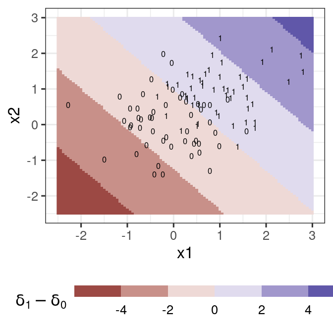
\[\delta_1(x)-\delta_0(x) = x^\top(a_1-a_0) + (b_1-b_0)\]

This is how we discriminate between the classes.

We just calculate \((a_1 - a_0)\) (a vector in \(\R^p\)), and \(b_1 - b_0\) (a scalar)

Baby example

library(mvtnorm)
library(MASS)
generate_lda_2d <- function(
    n, p = c(.5, .5), 
    mu = matrix(c(0, 0, 1, 1), 2),
    Sigma = diag(2)) {
  X <- rmvnorm(n, sigma = Sigma)
  tibble(
    y = which(rmultinom(n, 1, p) == 1, TRUE)[,1],
    x1 = X[, 1] + mu[1, y],
    x2 = X[, 2] + mu[2, y]
  )
}
dat1 <- generate_lda_2d(100, Sigma = .5 * diag(2))
lda_fit <- lda(y ~ ., dat1)

Multiple classes

moreclasses <- generate_lda_2d(150, c(.2, .3, .5), matrix(c(0, 0, 1, 1, 1, 0), 2), .5 * diag(2))
separateclasses <- generate_lda_2d(150, c(.2, .3, .5), matrix(c(-1, -1, 2, 2, 2, -1), 2), .1 * diag(2))

QDA

Just like LDA, but \(\Sigma_k\) is separate for each class.

Produces Quadratic decision boundary.

Everything else is the same.

qda_fit <- qda(y ~ ., dat1)
qda_3fit <- qda(y ~ ., moreclasses)

3 class comparison

Notes

• LDA is a linear classifier. It is not a linear smoother.
  • It is derived from Bayes rule.
  • Assume each class-conditional density in Gaussian
  • It assumes the classes have different mean vectors, but the same (common) covariance matrix.
  • It estimates densities and probabilities and “plugs in”
• QDA is not a linear classifier. It depends on quadratic functions of the data.
  • It is derived from Bayes rule.
  • Assume each class-conditional density in Gaussian
  • It assumes the classes have different mean vectors and different covariance matrices.
  • It estimates densities and probabilities and “plugs in”

It is hard (maybe impossible) to come up with reasonable classifiers that are linear smoothers. Many “look” like a linear smoother, but then apply a nonlinear transformation.

Naïve Bayes

Assume that \(Pr(X | Y = k) = Pr(X_1 | Y = k)\cdots Pr(X_p | Y = k)\).

That is, conditional on the class, the feature distribution is independent.

If we further assume that \(Pr(X_j | Y = k)\) is Gaussian,

This is the same as QDA but with \(\Sigma_k\) Diagonal.

Don’t have to assume Gaussian. Could do lots of stuff.

Next time…

Another linear classifier and transformations