The bootstrap
STAT 550
Daniel J. McDonald
\[\newcommand{\Expect}[1]{E\left[ #1 \right]} \newcommand{\Var}[1]{\mathrm{Var}\left[ #1 \right]} \newcommand{\Cov}[2]{\mathrm{Cov}\left[#1,\ #2\right]} \newcommand{\given}{\ \vert\ } \newcommand{\argmin}{\arg\min} \newcommand{\argmax}{\arg\max} \newcommand{\R}{\mathbb{R}} \newcommand{\P}{Pr} \renewcommand{\hat}{\widehat} \newcommand{\tr}[1]{\mbox{tr}(#1)} \newcommand{\X}{\mathbf{X}} \newcommand{\y}{\mathbf{y}}\]
In statistics…
The “bootstrap” works. And well.
It’s good for “second-level” analysis.
“First-level” analyses are things like \(\hat\beta\), \(\hat y\), an estimator of the center (a median), etc.
“Second-level” are things like \(\Var{\hat\beta}\), a confidence interval for \(\hat y\), or a median, etc.
You usually get these “second-level” properties from “the sampling distribution of an estimator”
But what if you don’t know the sampling distribution? Or you’re skeptical of the CLT argument?
Refresher on sampling distributions
- If \(X_i\) are iid Normal \((0,\sigma^2)\), then \(\Var{\bar{X}} = \sigma^2 / n\).
- If \(X_i\) are iid and \(n\) is big, then \(\Var{\bar{X}} \approx \Var{X_1} / n\).
- If \(X_i\) are iid Binomial \((m, p)\), then \(\Var{\bar{X}} = mp(1-p) / n\)
Example of unknown sampling distribution
I estimate a LDA on some data.
I get a new \(x_0\) and produce \(\hat{Pr}(y_0 =1 \given x_0)\).
Can I get a 95% confidence interval for \(Pr(y_0=1 \given x_0)\)?
The bootstrap gives this to you.
Procedure
- Resample your training data w/ replacement.
- Calculate a LDA on this sample.
- Produce a new prediction, call it \(\widehat{Pr}_b(y_0 =1 \given x_0)\).
- Repeat 1-3 \(b = 1,\ldots,B\) times.
- CI: \(\left[2\widehat{Pr}(y_0 =1 \given x_0) - \widehat{F}_{boot}(1-\alpha/2),\ 2\widehat{Pr}(y_0 =1 \given x_0) - \widehat{F}_{boot}(\alpha/2)\right]\)
\(\hat{F}\) is the “empirical” distribution of the bootstraps.
Very basic example
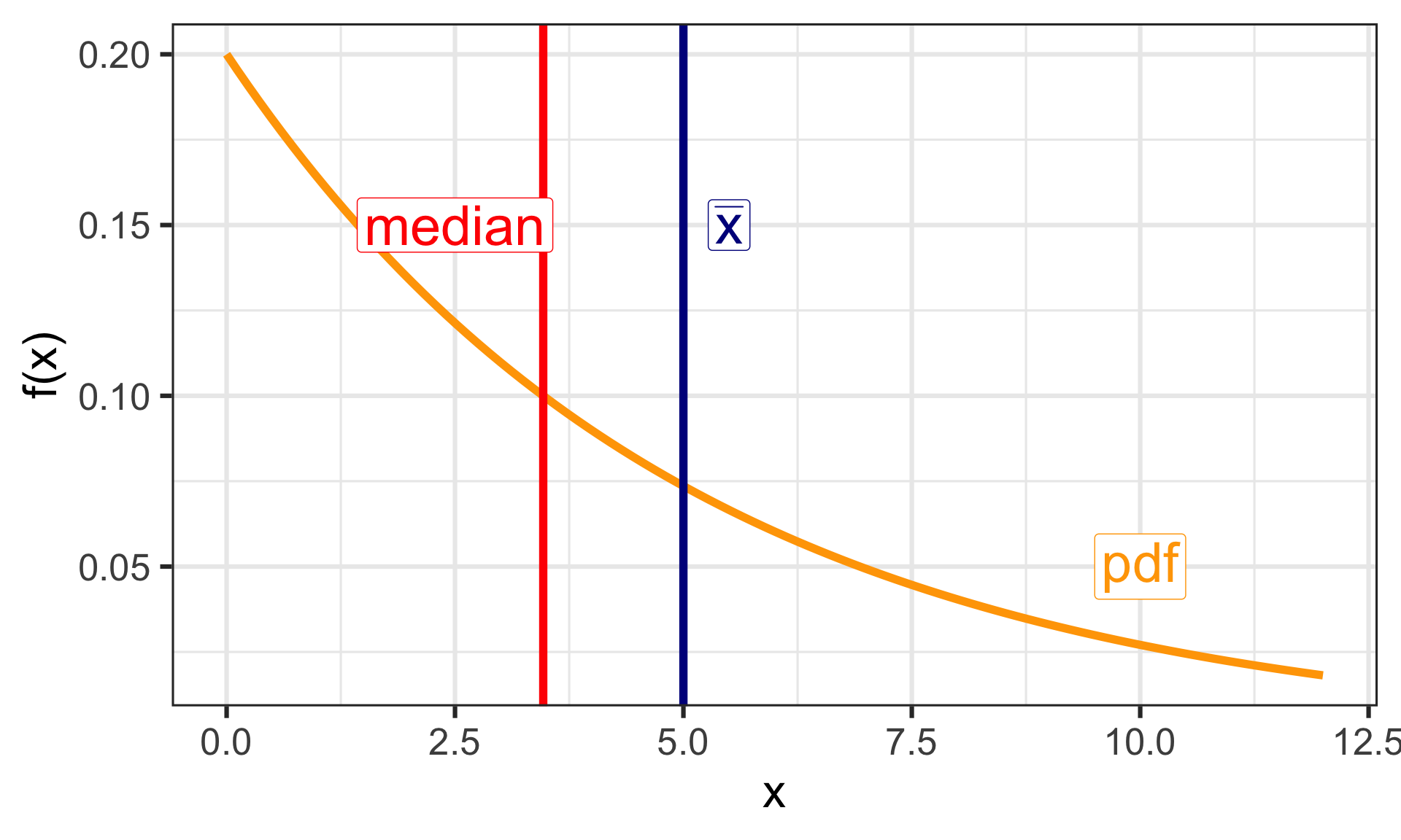
Let \(X_i\sim Exponential(1/5)\). The pdf is \(f(x) = \frac{1}{5}e^{-x/5}\)
I know if I estimate the mean with \(\bar{X}\), then by the CLT (if \(n\) is big),
\[\frac{\sqrt{n}(\bar{X}-E[X])}{s} \approx N(0, 1).\]
This gives me a 95% confidence interval like \[\bar{X} \pm 2 \frac{s}{\sqrt{n}}\]
But I don’t want to estimate the mean, I want to estimate the median.

Now what
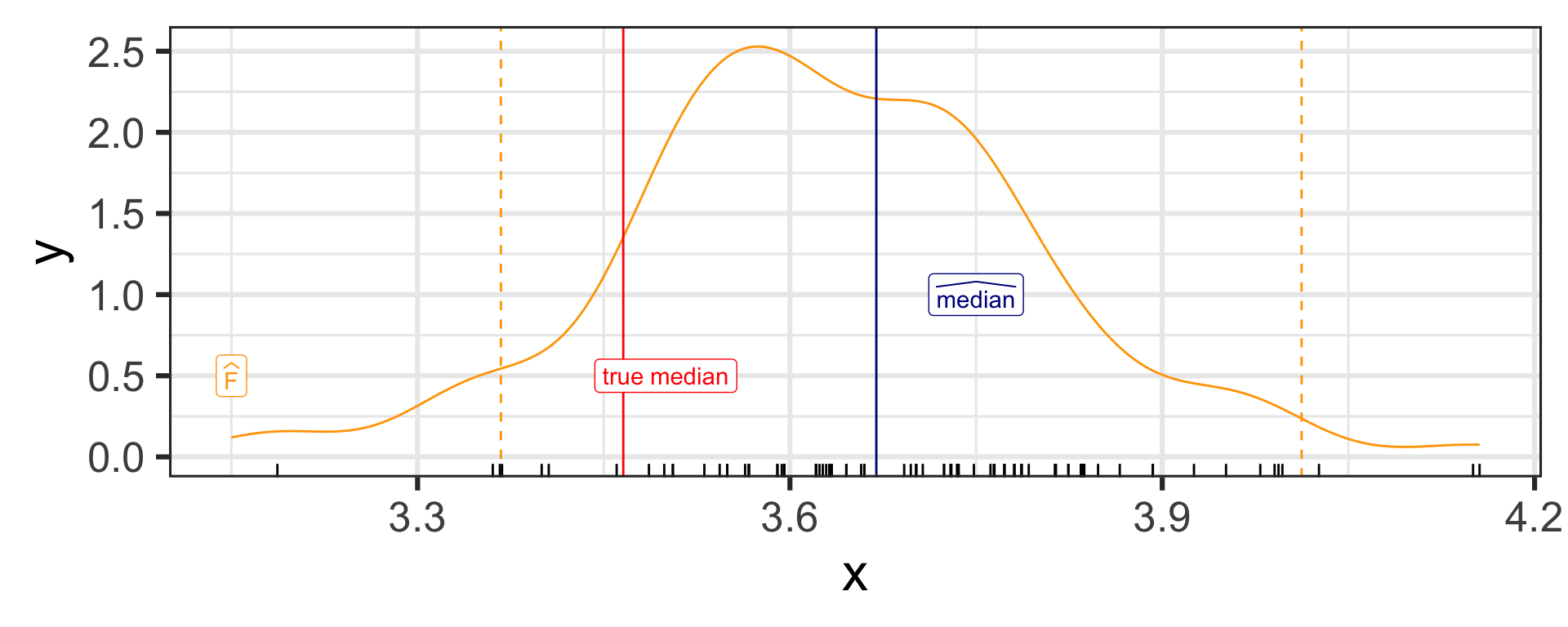
I give you a sample of size 500, you give me the sample median.
How do you get a CI?
You can use the bootstrap!
[1] 3.669627
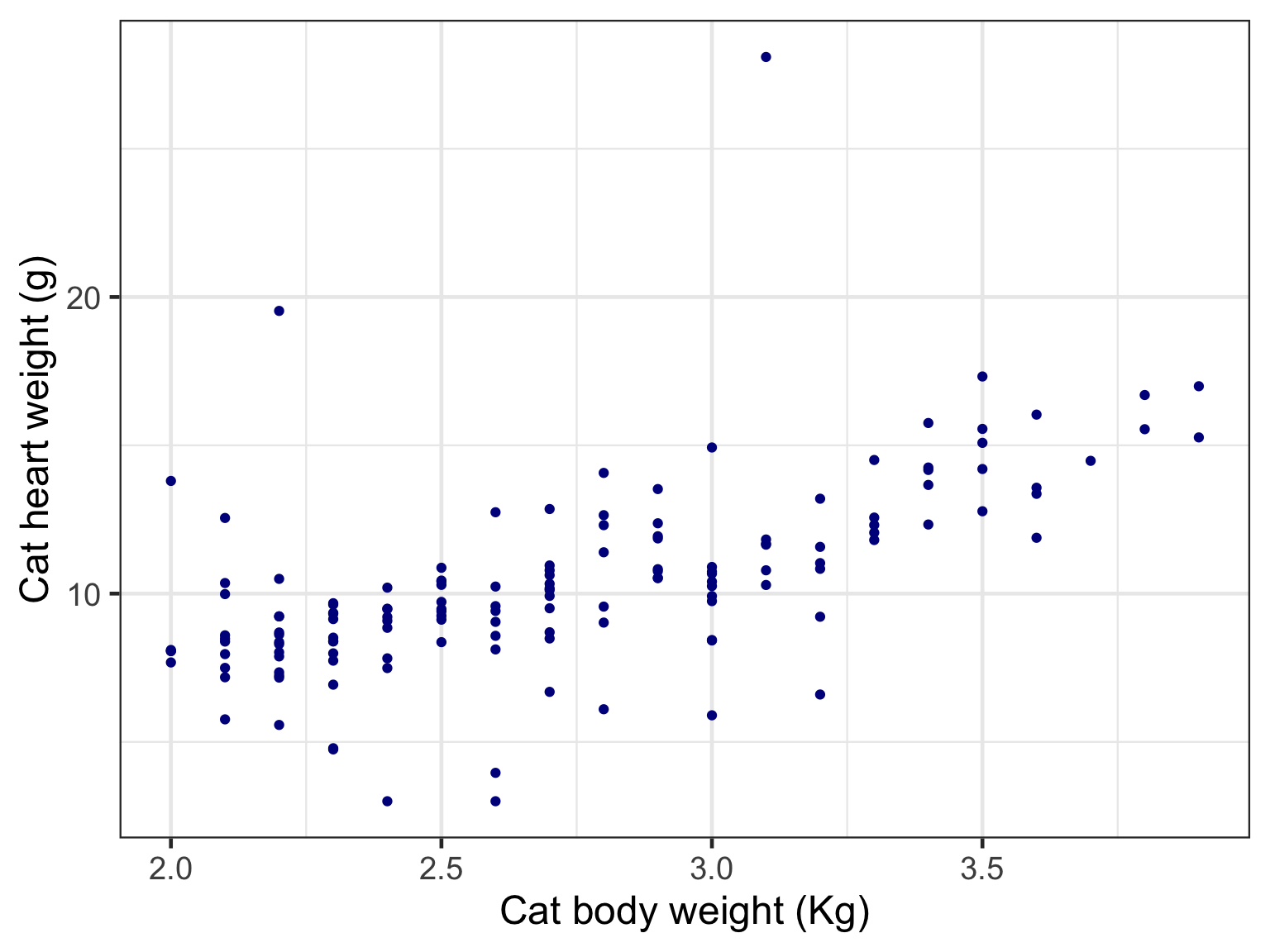
Slightly harder example

Call:
lm(formula = Hwt ~ 0 + Bwt, data = fatcats)

Residuals:
    Min      1Q  Median      3Q     Max
-6.9293 -1.0460 -0.1407  0.8298 16.2536

Coefficients:
    Estimate Std. Error t value Pr(>|t|)
Bwt  3.81895    0.07678   49.74   <2e-16 ***
---
Signif. codes:  0 '***' 0.001 '**' 0.01 '*' 0.05 '.' 0.1 ' ' 1

Residual standard error: 2.549 on 143 degrees of freedom
Multiple R-squared:  0.9454,    Adjusted R-squared:  0.945
F-statistic:  2474 on 1 and 143 DF,  p-value: < 2.2e-16
2.5 % 97.5 %
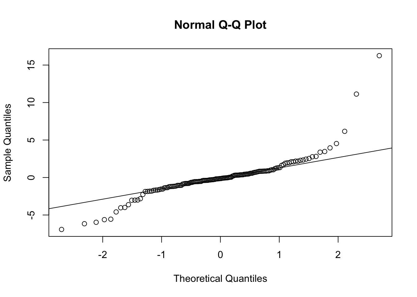
Bwt 3.667178 3.97073When we fit models, we examine diagnostics

The tails are too fat, I don’t believe that CI…
We bootstrap
B <- 500
bhats <- double(B)
alpha <- .05
for (b in 1:B) {
  samp <- sample(1:nrow(fatcats), replace = TRUE)
  newcats <- fatcats[samp, ] # new data
  bhats[b] <- coef(lm(Hwt ~ 0 + Bwt, data = newcats))
}

2 * coef(cats.lm) - # Bootstrap CI
  quantile(bhats, probs = c(1 - alpha / 2, alpha / 2))
97.5% 2.5%
3.654977 3.955927 2.5 % 97.5 %
Bwt 3.667178 3.97073An alternative
So far, I didn’t use any information about the data-generating process.
We’ve done the non-parametric bootstrap
This is easiest, and most common for most cases.
But there’s another version
You could try a “parametric bootstrap”
This assumes knowledge about the DGP
Same data
Non-parametric bootstrap
Same as before
B <- 500
bhats <- double(B)
alpha <- .05
for (b in 1:B) {
  samp <- sample(1:nrow(fatcats), replace = TRUE)
  newcats <- fatcats[samp, ] # new data
  bhats[b] <- coef(lm(Hwt ~ 0 + Bwt, data = newcats))
}

2 * coef(cats.lm) - # NP Bootstrap CI
  quantile(bhats, probs = c(1-alpha/2, alpha/2))
97.5% 2.5%
3.673559 3.970251 2.5 % 97.5 %
Bwt 3.667178 3.97073Parametric bootstrap
- Assume that the linear model is TRUE.
- Then, \(\texttt{Hwt}_i = \widehat{\beta}\times \texttt{Bwt}_i + \widehat{e}_i\), \(\widehat{e}_i \approx \epsilon_i\)
- The \(\epsilon_i\) is random \(\longrightarrow\) just resample \(\widehat{e}_i\).
B <- 500
bhats <- double(B)
alpha <- .05
cats.lm <- lm(Hwt ~ 0 + Bwt, data = fatcats)
newcats <- fatcats
for (b in 1:B) {
  samp <- sample(residuals(cats.lm), replace = TRUE)
  newcats$Hwt <- predict(cats.lm) + samp # new data
  bhats[b] <- coef(lm(Hwt ~ 0 + Bwt, data = newcats))
}

2 * coef(cats.lm) - # Parametric Bootstrap CI
  quantile(bhats, probs = c(1 - alpha/2, alpha/2))
97.5% 2.5%
3.665531 3.961896 Bootstrap error sources
Simulation error:
using only \(B\) samples to estimate \(F\) with \(\hat{F}\).
Statistical error:
our data depended on a sample from the population. We don’t have the whole population so we make an error by using a sample
(Note: this part is what always happens with data, and what the science of statistics analyzes.)
Specification error:
If we use the parametric bootstrap, and our model is wrong, then we are overconfident.