At time \(i\), we observe the sum of all past noise
\[y_i = \sum_{j=-\infty}^0 a_{i+j} \epsilon_j\]
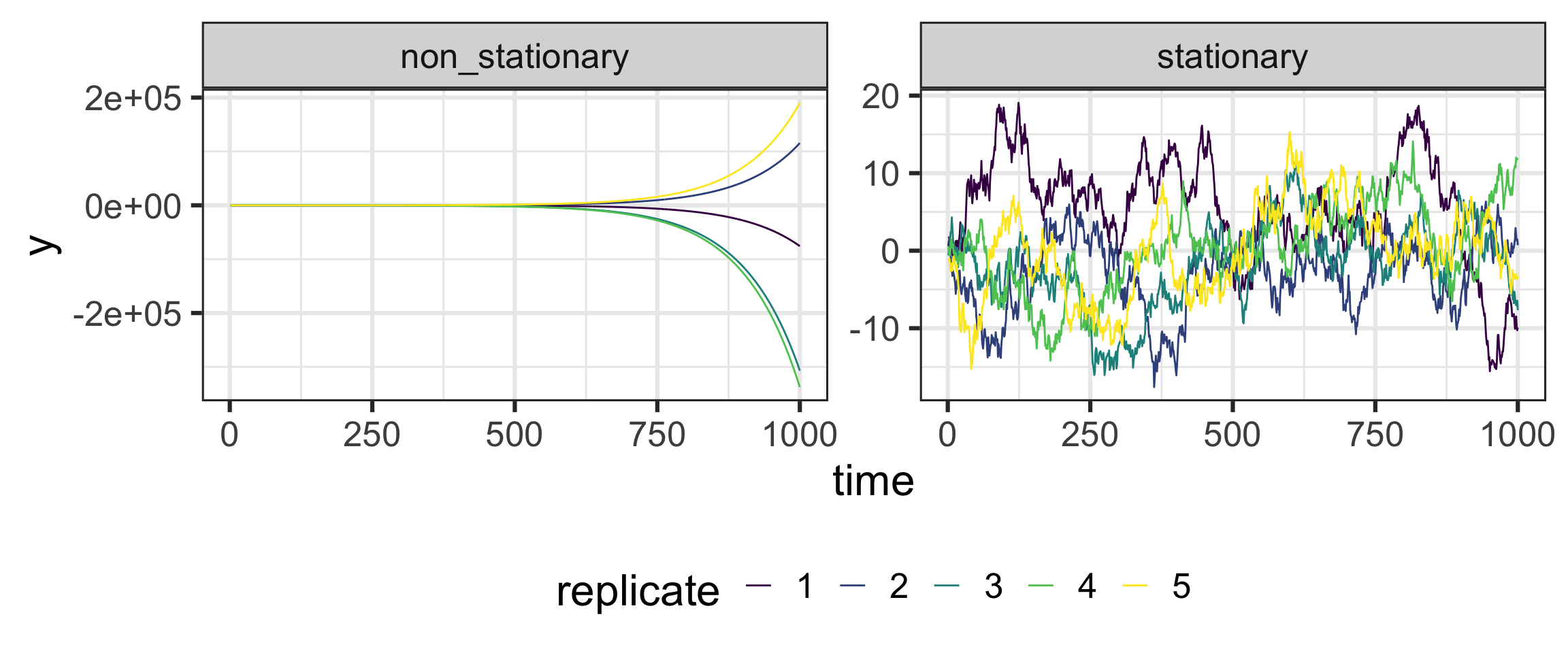
Without some conditions on \(\{a_k\}_{k=-\infty}^0\) this process will “run away”
The result is “non-stationary” and difficult to analyze.
Stationary means (roughly) that the marginal distribution of \(y_i\) does not change with \(i\).
Chasing stationarity
n <-1000set.seed(12345)nseq <-5generate_ar <-function(id, n, b) { y <-double(n) y[1] <-rnorm(1)for (i in2:n) y[i] <- b * y[i -1] +rnorm(1)tibble(time =1:n, y = y, id = id)}stationary <-map_dfr(1:nseq, ~generate_ar(.x, n = n, b = .99))non_stationary <-map_dfr(1:nseq, ~generate_ar(.x, n = n, b =1.01))
Uses of stationarity
Lots of types (weak, strong, in-mean, wide-sense,…)
not required for modelling / forecasting
But assuming stationarity gives some important guarantees
Usually work with stationary processes
Standard models
AR(p)
Suppose \(\epsilon_i\) are i.i.d. N(0, 1) (distn is convenient, but not required)
Now \(X\) is a \(q\)-dimensional AR(1) (but we don’t see it)
\(y\) is deterministic conditional on \(X\)
This is the usual way these are estimated using a State-Space Model
Many time series models have multiple equivalent representations
ARIMA
We’ve been using arima() and arima.sim(), so what is left?
The “I” means “integrated”
If, for example, we can write \(z_i = y_i - y_{i-1}\) and \(z\) follows an ARMA(p, q), we say \(y\) follows an ARIMA(p, 1, q).
The middle term is the degree of differencing
Other standard models
Suppose we can write
\[
y_i = T_i + S_i + W_i
\]
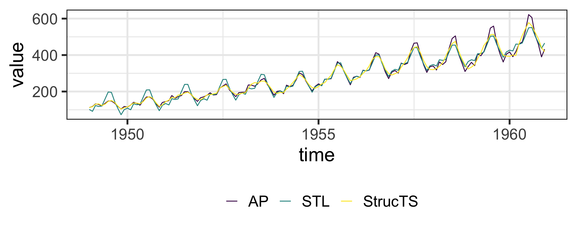
This is the “classical” decomposition of \(y\) into a Trend + Seasonal + Noise.
You can estimate this with a “Basic Structural Time Series Model” using StrucTS().
A related, though slightly different model is called the STL decomposition, estimated with stl().
This is “Seasonal Decomposition of Time Series by Loess”
(LOESS is “locally estimated scatterplot smoothing” named/proposed independently by Bill Cleveland though originally proposed about 15 years earlier and called the Savitsky-Golay Filter)
Quick example
sts <-StructTS(AirPassengers)bc <-stl(AirPassengers, "periodic") # use sin/cos to represent the seasonaltibble(time =seq(as.Date("1949-01-01"), as.Date("1960-12-31"), by ="month"),AP = AirPassengers, StrucTS =fitted(sts)[,1], STL =rowSums(bc$time.series[,1:2])) %>%pivot_longer(-time) %>%ggplot(aes(time, value, color = name)) +geom_line() +theme_bw(base_size =24) +scale_color_viridis_d(name ="") +theme(legend.position ="bottom")
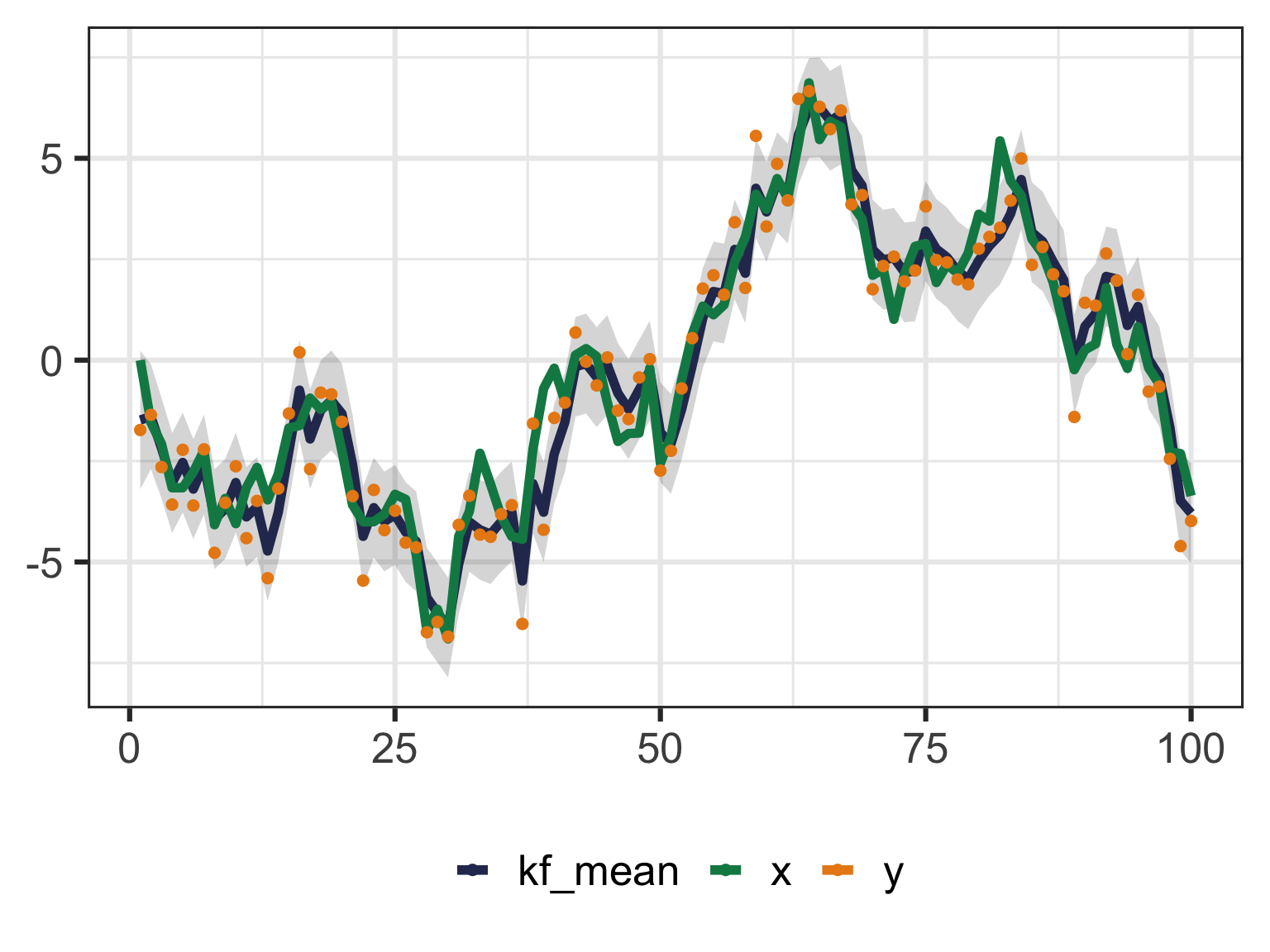
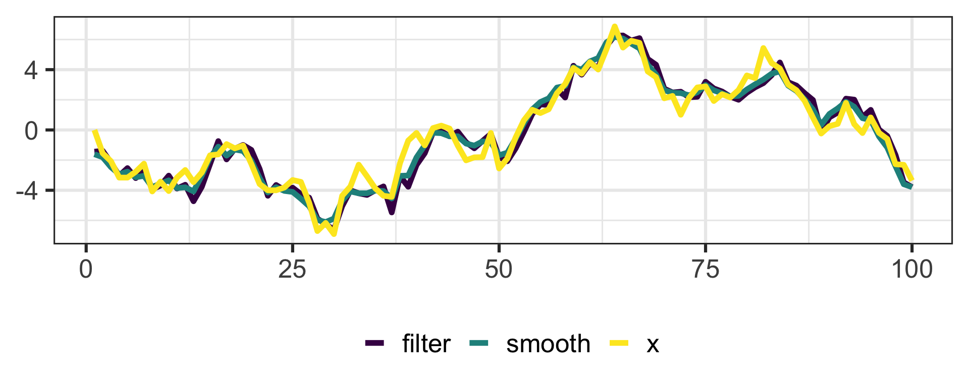
kalman <-function(y, m0, P0, A, Q, H, R) { n <-length(y) m <-double(n+1) P <-double(n+1) m[1] <- m0 P[1] <- P0for (k inseq(n)) { mm <- A * m[k] Pm <- A * P[k] * A + Q v <- y[k] - H * mm S <- H * Pm * H + R K <- Pm * H / S m[k+1] <- mm + K * v P[k+1] <- Pm - K * S * K }tibble(t =1:n, m = m[-1], P = P[-1])}set.seed(2022-06-01)x <-double(100)for (k in2:100) x[k] = x[k -1] +rnorm(1)y <- x +rnorm(100, sd =1)kf <-kalman(y, 0, 5, 1, 1, 1, 1)
Important notes
So far, we assumed all parameters were known.
In reality, we had 6: m0, P0, A, Q, H, R
I sort of also think of x as “parameters” in the Bayesian sense
By that I mean, “latent variables for which we have prior distributions”
What if we want to estimate them?
Bayesian way: m0 and P0 are already the parameters of for the prior on x1. Put priors on the other 4.
Frequentist way: Just maximize the likelihood. Can technically take P0\(\rightarrow\infty\) to remove it and m0
The Likelihood is produced as a by-product of the Kalman Filter.