Principal components analysis
Stat 550
Daniel J. McDonald
Last modified – 03 April 2024
\[
\DeclareMathOperator*{\argmin}{argmin}
\DeclareMathOperator*{\argmax}{argmax}
\DeclareMathOperator*{\minimize}{minimize}
\DeclareMathOperator*{\maximize}{maximize}
\DeclareMathOperator*{\find}{find}
\DeclareMathOperator{\st}{subject\,\,to}
\newcommand{\E}{E}
\newcommand{\Expect}[1]{\E\left[ #1 \right]}
\newcommand{\Var}[1]{\mathrm{Var}\left[ #1 \right]}
\newcommand{\Cov}[2]{\mathrm{Cov}\left[#1,\ #2\right]}
\newcommand{\given}{\mid}
\newcommand{\X}{\mathbf{X}}
\newcommand{\x}{\mathbf{x}}
\newcommand{\y}{\mathbf{y}}
\newcommand{\P}{\mathcal{P}}
\newcommand{\R}{\mathbb{R}}
\newcommand{\norm}[1]{\left\lVert #1 \right\rVert}
\newcommand{\snorm}[1]{\lVert #1 \rVert}
\newcommand{\tr}[1]{\mbox{tr}(#1)}
\newcommand{\U}{\mathbf{U}}
\newcommand{\D}{\mathbf{D}}
\newcommand{\V}{\mathbf{V}}
\renewcommand{\hat}{\widehat}
\]
Representation learning
Representation learning is the idea that performance of ML methods is highly dependent on the choice of representation
For this reason, much of ML is geared towards transforming the data into the relevant features and then using these as inputs
This idea is as old as statistics itself, really,
However, the idea is constantly revisited in a variety of fields and contexts
Commonly, these learned representations capture low-level information like overall shapes
It is possible to quantify this intuition for PCA at least
- Goal
-
Transform \(\mathbf{X}\in \R^{n\times p}\) into \(\mathbf{Z} \in \R^{n \times ?}\)
?-dimension can be bigger (feature creation) or smaller (dimension reduction) than \(p\)
PCA
Principal components analysis (PCA) is a dimension reduction technique
It solves various equivalent optimization problems
(Maximize variance, minimize \(\ell_2\) distortions, find closest subspace of a given rank, \(\ldots\))
At its core, we are finding linear combinations of the original (centered) data \[z_{ij} = \alpha_j^{\top} x_i\]
![]()
Lower dimensional embeddings
Suppose we have predictors \(\x_1\) and \(\x_2\) (columns / features / measurements)
- We more faithfully preserve the structure of this data by keeping \(\x_1\) and setting \(\x_2\) to zero than the opposite
![]()
Lower dimensional embeddings
An important feature of the previous example is that \(\x_1\) and \(\x_2\) aren’t correlated
What if they are?
![]()
We lose a lot of structure by setting either \(\x_1\) or \(\x_2\) to zero
Lower dimensional embeddings
The only difference is the first is a rotation of the second
![]()
PCA
If we knew how to rotate our data, then we could more easily retain the structure.
PCA gives us exactly this rotation
- Center (+scale?) the data matrix \(\X\)
- Compute the SVD of \(\X = \U\D \V^\top\) (always exists)
- Return \(\U_M\D_M\), where \(\D_M\) is the largest \(M\) singular values of \(\X\)
PCA
![]()
PCA on some pop music data
# A tibble: 1,269 × 15
   artist      danceability energy   key loudness  mode speechiness acousticness
   <fct>              <dbl>  <dbl> <int>    <dbl> <int>       <dbl>        <dbl>
 1 Taylor Swi…        0.781  0.357     0   -16.4      1      0.912       0.717
 2 Taylor Swi…        0.627  0.266     9   -15.4      1      0.929       0.796
 3 Taylor Swi…        0.516  0.917    11    -3.19     0      0.0827      0.0139
 4 Taylor Swi…        0.629  0.757     1    -8.37     0      0.0512      0.00384
 5 Taylor Swi…        0.686  0.705     9   -10.8      1      0.249       0.832
 6 Taylor Swi…        0.522  0.691     2    -4.82     1      0.0307      0.00609
 7 Taylor Swi…        0.31   0.374     6    -8.46     1      0.0275      0.761
 8 Taylor Swi…        0.705  0.621     2    -8.09     1      0.0334      0.101
 9 Taylor Swi…        0.553  0.604     1    -5.30     0      0.0258      0.202
10 Taylor Swi…        0.419  0.908     9    -5.16     1      0.0651      0.00048
# ℹ 1,259 more rows
# ℹ 7 more variables: instrumentalness <dbl>, liveness <dbl>, valence <dbl>,
#   tempo <dbl>, time_signature <int>, duration_ms <int>, explicit <lgl>
PCA on some pop music data
- 15 dimensions to 2
- coloured by artist
![]()
Plotting the weights, \(\alpha_j,\ j=1,2\)
![]()
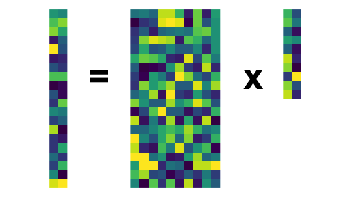
Matrix decompositions
At its core, we are finding linear combinations of the original (centered) data \[z_{ij} = \alpha_j^{\top} x_i\]
This is expressed via the SVD: \(\X = \U\D\V^{\top}\).
We assume throughout that we have centered the data
Then our new features are
\[\mathbf{Z} = \X \V = \U\D\]
Short SVD aside
Any \(n\times p\) matrix can be decomposed into \(\mathbf{UDV}^\top\).
This is a computational procedure, like inverting a matrix, svd()
These have properties:
- \(\mathbf{U}^\top \mathbf{U} = \mathbf{I}_n\)
- \(\mathbf{V}^\top \mathbf{V} = \mathbf{I}_p\)
- \(\mathbf{D}\) is diagonal (0 off the diagonal)
Many methods for dimension reduction use the SVD of some matrix.
Why?
Given \(\X\), find a projection \(\mathbf{P}\) onto \(\R^M\) with \(M \leq p\) that minimizes the reconstruction error \[
\begin{aligned}
\min_{\mathbf{P}} &\,\, \lVert \mathbf{X} - \mathbf{X}\mathbf{P} \rVert^2_F \,\,\, \textrm{(sum all the elements)}\\
\textrm{subject to} &\,\, \textrm{rank}(\mathbf{P}) = M,\, \mathbf{P} = \mathbf{P}^T,\, \mathbf{P} = \mathbf{P}^2
\end{aligned}
\] The conditions ensure that \(\mathbf{P}\) is a projection matrix onto \(M\) dimensions.
Maximize the variance explained by an orthogonal transformation \(\mathbf{A} \in \R^{p\times M}\) \[
\begin{aligned}
\max_{\mathbf{A}} &\,\, \textrm{trace}\left(\frac{1}{n}\mathbf{A}^\top \X^\top \X \mathbf{A}\right)\\
\textrm{subject to} &\,\, \mathbf{A}^\top\mathbf{A} = \mathbf{I}_M
\end{aligned}
\]
- In case one, the minimizer is \(\mathbf{P} = \mathbf{V}_M\mathbf{V}_M^\top\)
- In case two, the maximizer is \(\mathbf{A} = \mathbf{V}_M\).