Lecture 5: Tidy Data and the Tidyverse
STAT 545 - Fall 2025
Today’s Goals
recognize whether a given data set is ‘tidy’ or ‘untidy’ for their analysis
understand why ‘tidy’ data can be useful
reshape a data set between ‘long’ and ‘wide’ formats, using
tidyr::pivot_longer()andtidyr::pivot_wider()understand how to grapple with explicit missing values created by pivoting
Quick links:
Required Packages
Install (if necessary) and load in the following packages:
The Tidyverse
a “meta”-package that contains a bunch of packages related to tidy data!
includes
dplyr,ggplot2,tidyr(today’s topic) and more
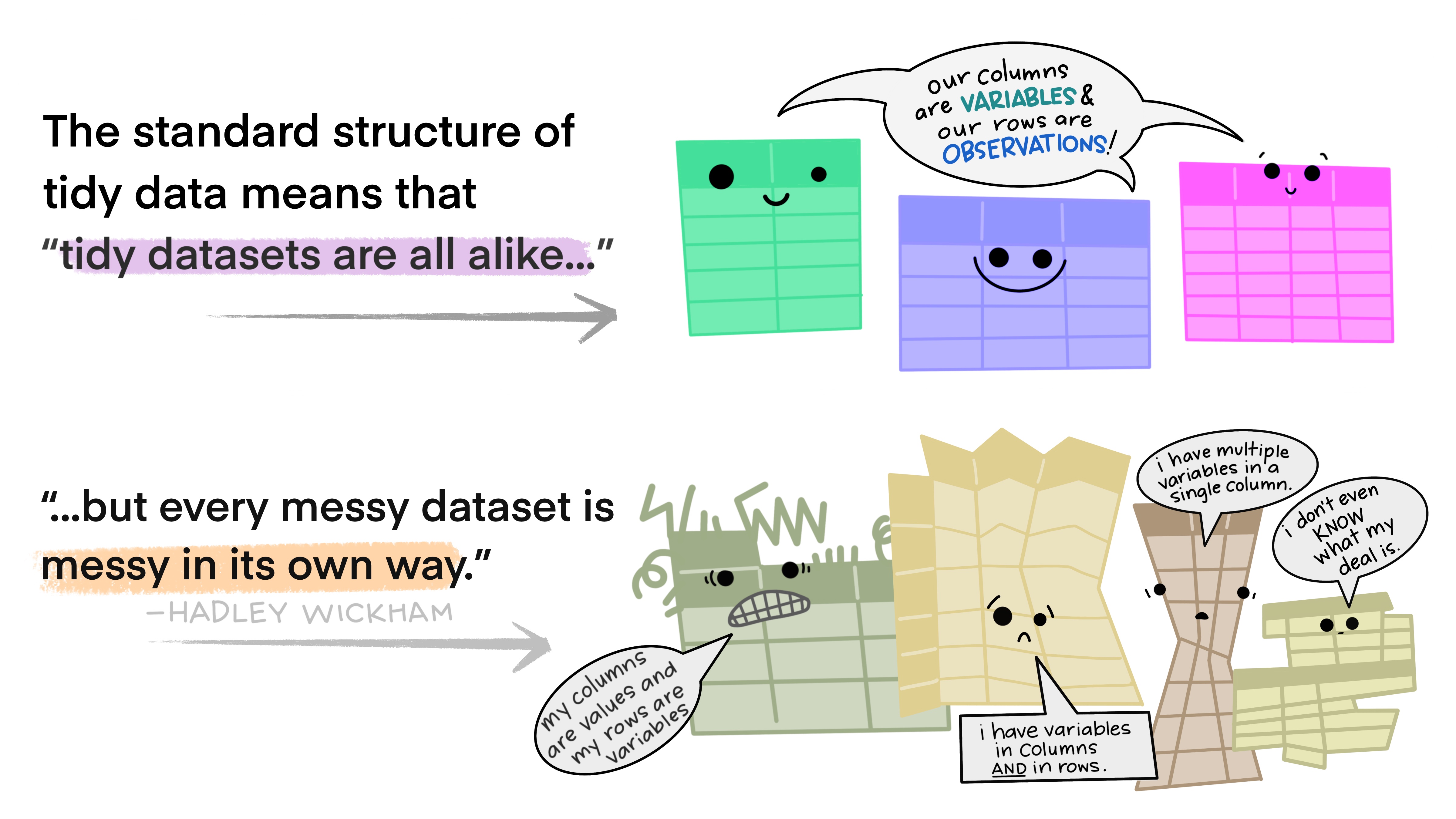
What is “Tidy Data”?
Tidy data is defined as data where
each variables form a column,
each observation forms a row, and
each cell is a single measurement
What constitutes a variable, observation, and measurement will depend on the goal of your analysis!
When we have tidy data, it makes our lives easier.
What is “Tidy Data”?
Artwork by Allison Horst (@allisonhorst)
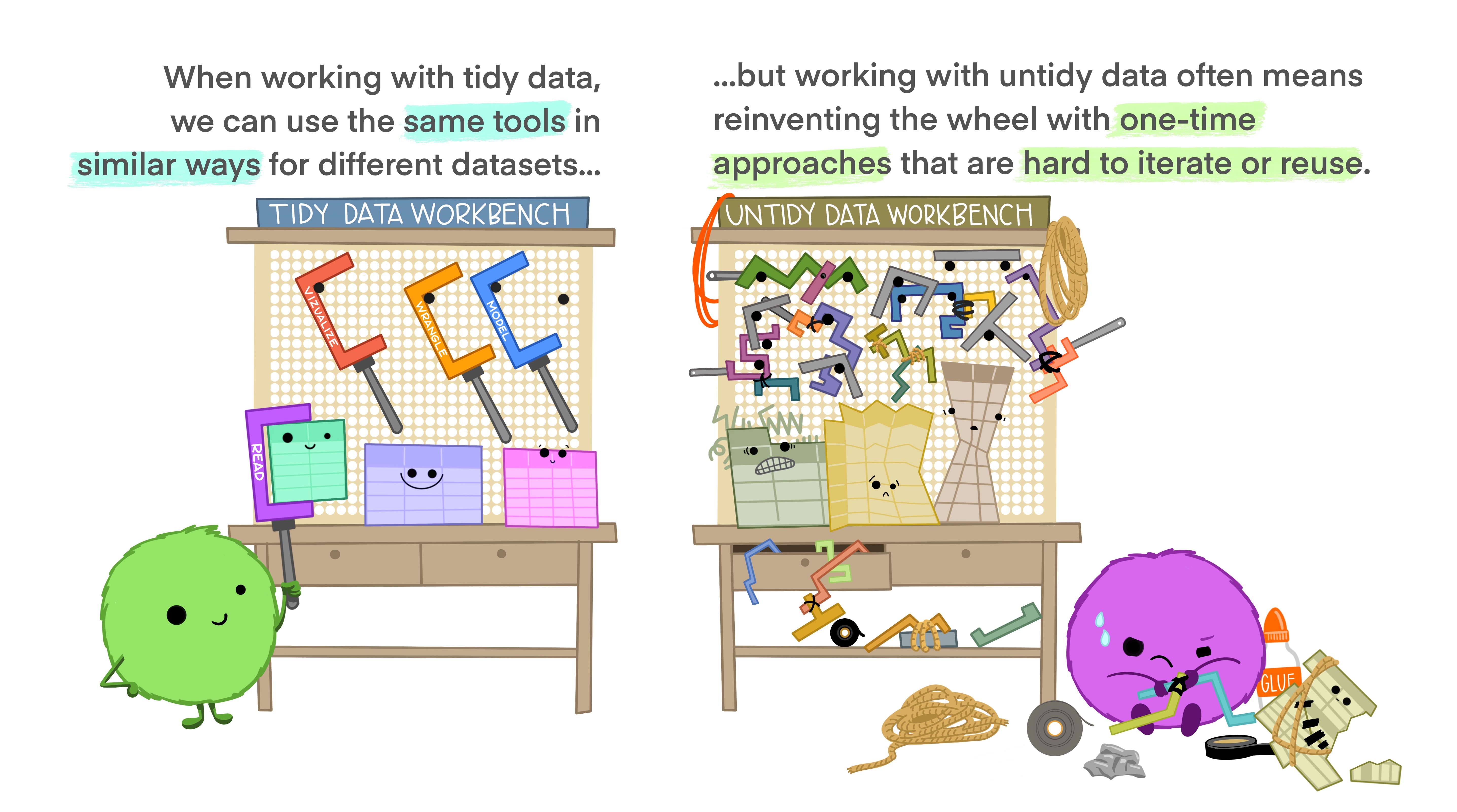
Why Tidy Data?
Artwork by Allison Horst (@allisonhorst)
Untidy Real Data Example
Tidy Data Example
Discussion #1: Drinks
The fivethirtyeight R package contains a dataset called drinks. This dataset was compiled as part of a FiveThirtyEight article that explored (among other things) which countries consumes the most alcohol. Let’s look at a subset of the data:
If we wanted to compare consumption across countries by drink type, is the data tidy?
Notes:
Discussion #2: Drinks
The following graphic was made from the same drinks dataset.
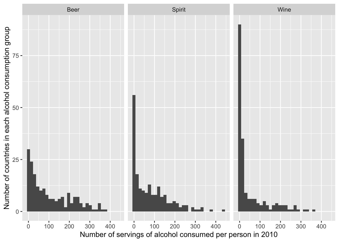
Without transforming the data (on previous slide), would we be able to plot this?
Notes:
Basic Pivoting
Once you have figured out what’s tidy for you, you may come to realize that your data is not tidy. As we have discussed, it will typically save you time and frustration to tidy it before moving on in your analysis.
Very often this will involve using “pivoting” type functions. For example, the tidyr package in the tidyverse has two main pivoting functions:
pivot_longer()makes datasets longer: it moves some information in the columns into new rows, thereby increasing the number of rows of the dataset.pivot_wider()makes datasets wider: it moves some information in the rows into new columns, thereby decreasing the number of rows of the dataset.
Pivoting Wider
Here is an example of (artificial) data that is currently in “long” format, looking grades before and after active learning was incorporated into their math and science lectures:
Sometimes, we require data involving time to have row for each observation, and one column for each time point (i.e., wide data). While this isn’t our “standard” definition of tidy, sometimes this is what is required for longitudinal data (i.e., data involving measures repeated over time). Nevertheless, let’s try to pivot this table!
Pivoting Wider
pivot_wider needs three pieces of information:
What is a set of columns that uniquely identifies each observation? Put their names in the
id_colsargument.Where should the names for the new columns come from? Put the name of the column you want to take the new variable names from in the
names_fromargument.What values should the new columns contain? Put the name of the columns you want to take the values from to
values_fromin thevalues_fromargument.
Note that if you don’t specify an id_cols argument, pivot_wider will assume that you want it to be every column except those in names_from and values_from. Further, any columns not included in id_cols, names_from, and values_from (e.g., ep_id) will simply be dropped.
Pivoting Wider: Grades Example
Recall the structure of grades_long:
Can you pivot this table wider so that we have a columns “Scores_Before” and “Scores_After” for each student_id and subject?
Pivoting Longer
Here is a snippet of WHO data on the number of tuberculosis cases in different years in different countries.
If we wanted to compare tuberculosis cases over time by country (e.g. by plotting the year on the x-axis and case count on the y-axis with a line for each country), then this format is not tidy. there should be one observation per unit within each population (country-years).
In this case, we do not observe units within each country-year, so each observation is a country-year. The variables then fall into place: the country and year labels, and the case counts.
Tidy Format: variables (the year, the country, and the case counts) on the columns. There are 6 rows, one for each unique country-year combination. In this example, the tidy format is longer. That means to produce it using who_wide, we need to lengthen it by moving some information in the column names (the info about the measurement year) into new rows.
Pivoting Longer
pivot_longer needs three pieces of information:
Which are the columns that we want to expand into more rows? Put their names in the
colsargument.We want to save the information in the names of those columns as values in new column(s) of our dataset. What should we name these new column(s)? This is the
names_toargument.We also want to preserve the information in the values of those columns - so we should save them as values in a new column of our dataset. What should we name it? This is the
values_toargument.
Pivoting Longer: WHO Example
Now we’ve got tidy data!
Pivoting Longer: Grades Example
Challenge yourself to transform grades_wide back to grades_long. Rename your new dataset grades_long_pivoted and compare the two long forms.
Pivoting Longer with Multiple Variables: WHO Example
Example: Column Names Contain Multiple Variable Values
Here’s a more realistic (but still simplified) look at the WHO Tuberculosis data.
This time, cases are broken down by gender (f or m only considered in this study) and by age range (014 (0 - 14), 1524 (15 - 24), 2534 (25 - 34), and so on)
Suppose now that we are interested in comparing tuberculosis rates over time across (potentially) gender, age, and country. Then the most granular population we are trying to describe is a country, gender, age, and year combination, and like in the last example, we have no measured sub-units within that population, so an observation is a unique combination of country, gender, age, and year. (What a mouthful!)
Pivoting Longer with Multiple Variables: WHO Example
Variables of interest: country, year, gender, age range, and case count.
Values for gender and age range are currently located in the column names of who_demo, and values for case count are currently spread across multiple columns. So to tidy who_demo up, we need to use pivot_longer() to move the info in the columns into new rows.
Phew!
Separating and Uniting
Sometimes data has multiple pieces of information stored in a single column. To separate them into two distinct columns, we can use the separate() function from the tidyverse (technically, a package within tidyverse called tidyr.
separate(): separates information within a column. It involves three arguments:
col: specifies the column we want to separateinto: specifies the names of the new columns.sep: specifies where we want to cut. The default is pretty clever - it separates at any non-alphanumeric value. (How this is accomplished involves regular expressions, which are very useful when working with character data. We will learn more about regular expressions in STAT 545B. )
Separating and Uniting
Conversely, unite() combines information from two or more columns into one. Involves:
col: name of the new column...: the names of columns to be unitedsep: specifies the separator to use between values (i.e., “-”)
Separating and Uniting: WHO Example
The tidyr package has a function for gluing columns together (unite) and for cutting columns apart (separate). Why might this help us tidy? Here is another snippet of WHO Tuberculosis data.
The rate column contains the values of two variables: case counts and population counts. We would like to snip it apart at the “/” character to create two columns:
Untidy Data
As we’ve seen, tidy data is often very helpful. But there are also times when untidy data is good. Here are a few reasons:
The format that lends itself best to fast computations might not be tidy. Case Study: Tidy Genomics.
Untidy data is often easier for humans to interpret and edit. See Untidy Data: The Unreasonable Effectiveness of Tables.
We could lose important information about the context in which the data was collected by cleaning and tidying raw data. This can have important ethical implications; see Chapter 5 of the book “Data Feminism” by Catherine D’Ignazio and Lauren F. Klein.
In summary, tidiness is a very useful concept, and tidying data is often useful. But we should remember that absolutes are few and far between in data science and statistics. Just because tidying data is often useful, doesn’t mean it’s always useful.
Worksheet A4
We will spend the remainder of this class and Thursday’s class (TAs only) working through Worksheet A4.
To Save These Slides With Your Code
To Print to PDF (with your code!), do the following:
Open the in-browser print dialog
CMD/CTRL + Por Right click > PrintChange the Destination setting to Save as PDF.
Change the Layout to Landscape.
Change the Margins to None. Enable the Background graphics option.
Click Save 🎉
In all cases, ensure the code chunks don’t get cut off (i.e., a line is too long). You will not be able to edit these from the PDF directly (though you could open the slides again and copy-and-paste to re-run the code!)