Linear Regression Framework
Contents
Overview
In the previous chapters we introduced A/B testing experiments, highlighted some common problems encounter in real applications and examined some potential solutions. A/B testing experiments are commonly used to examine the effect of variations in products or services on a variable of interest. For example, a company may want to know if using a different picture in the home page of their website increases their online sales. However, there are many other variables that probably affect the sales of the company.
A/B testing experiment can not be used to study the relation between continous variables. For example, is the montly investment in advertisement related with the sales of the company? Alternatively, a linear regression can be used to examine the relation of variables with a continuous response. Linear regression model can include different types of input variables, including categorical variables. Thus, many of the concepts learned in A/B testing can be thought as particular cases of linear regression models. In this chapter, we introduce linear regression models, discuss their scope, and present the least squares estimation method.
Historical throwback …
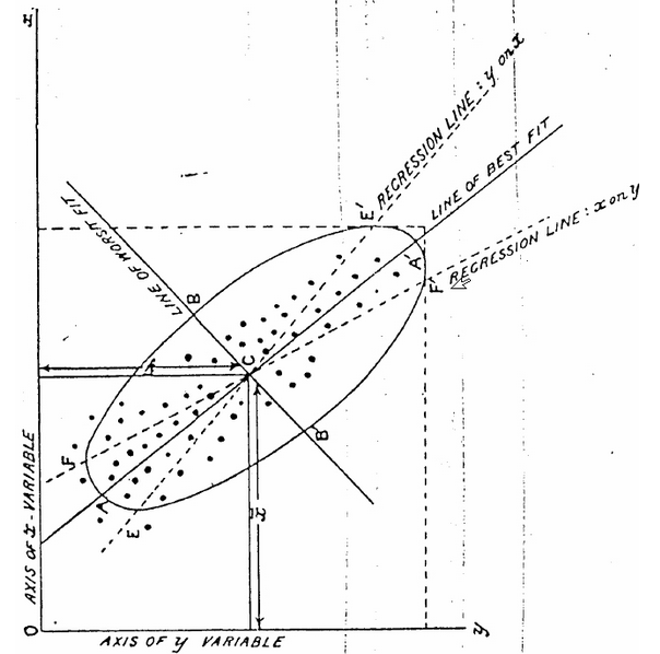
Least squares (LS) method was first used by Legendre (1805) and by Gauss (1809) to estimate the orbits of comets based on measurements of the comets’ previous locations. Gauss even predicted the appearence of the asteroid Ceres using LS combined with other complex computations. However, neither Legendre or Gauss coined the term “Regression”. Francis Galton in the nineteenth century used this term to describe a biological phenomenon that he observed: “It appeared from these experiments that the offspring did not tend to resemble their parents seeds in size, but to be always more mediocre than they”. Unfortunately, Francis Galton had disturbing and unacceptable views of race. Later, his colleague Karl Pearson associated LS method to regression. He observed that in the plot of the heights of parents on the x-axis and their children on the y-axis, the slope of the LS line was smaller than one. He named the LS line as the regression line. R.A. Fisher later combined the work of Gauss and Pearson and studied the theoretical properties of LS estimators for Regression.
A full story can be found in The Discovery of Statistical Regression.

|
 |
Generative vs Predictive models
Linear regression models provide a unifying framework to estimate and test the true relation between different type of variables and a continuous response. These linear models can also be used to predict the value of a continuous response (although it may not be the best predictive model). Different methods can be used to estimate and evaluate linear models depending on the primary goal of the study.
Models can be classified as generative models, when the primary goal is to understand the model that generates the data, or predictive models, when the primary goal is to predict the response value of a new case that was not seen by the estimated model. Let’s see some examples.
Generative models
As data scientists, you are often interested in understanding the model that generates the data. For example:
which variables are associated with a response of interest?
can we model the relationship between the response and the input variables? Is a linear model adequate?
which variables are positively/negatively associated with the response?
does the relationship between the response and an input variable depend on the values of the other variables?
Examples in generative models:
A real estate agent wants to identify factors that are related to the assessed values of homes (e.g., size of houses, age, amenities, etc)
Biologists want to verify empirically the central dogma of biology that relates mRNA values to protein values in living organisms
Predictive models
As data scientists, you are also interested in predicting the response value of a new case that was not seen by the estimated model. For example:
can we predict the response variables using a linear model?
what would be the response for a future observation in our study?
which input variables are best to predict the response?
Examples in prediction models:
A real estate agent is interested in determining if a house is under- or over-valued given its characteristics (prediction problem)
Biologists want to use mRNA data to predict protein values
Linear regression models can be used to answer any of these questions.
Linear regression in real applications
How have linear regression models been used? Given its simple form, linear models have been widely used to study the relation between variables and to build predictive models. We reviewed some examples below:
Medicine and Molecular Biology: an example of prediction
Scientists have used simple linear regression models to quantitatively explain the Central Dogma of Biology. This article, published in Nature (2017, 547:E19–E20), Can We Predict Protein from mRNA levels?, highlights the missused of correlation studies in this context.

Climate Change: an example of estimation and inference
Economists have used different linear regression models to explain people’s choices in relation to climate variables. Reference: JAERE 2016; 3(1): 205-246. A featured article in FiveThirtyEight tells more about this study: Here’s The Best Place To Move If You’re Worried About Climate Change

Sports: an example of prediction
Billy Bean, manager of the Oakland Athletics, used statistics to identify low cost players who can help the team win (example from Advanced Data Science, Rafael Irizarry).
 |
 |
Case Study: California Schools
We will use a real world dataset called CASchools that contains data from 420 school districts in California available for 1998 and 1999. The data set comes with an R package called AER, an acronym for Applied Econometrics with R (by Christian Kleiber & Zeileis, 2017). Test scores are on the Stanford 9 standardized test administered to 5th grade students. School characteristics and demographic variables for the students are averaged across the district.
Question
We want to examine which demographic variables and school characteristics are associated with the performance of the students.
The following variables are available in this dataset for each district:
district: district codeenglish: percentage of students in the district that are English learners, i.e., students for whom English is a second languageread: average reading scoremath: average math scorestudents: total enrollmentteachers: number of teacherscalworks: percent qualifying for CalWorks (income assistance)lunch: percent qualifying for reduced-price lunchcomputer: number of computersexpenditure: expenditure per studentincome: district average income (in USD 1,000)english: percent of English learners
We will construct 2 new variables that will help us respond to the question of interest:
score: average math and reading scoresstratio: ratio of the number of students to the number of teachers
Linear Regression Framework
Mathematically, a general framework for a multiple linear regression can be written as:
where \(E(\varepsilon_i|X_{1i}, \ldots, X_{pi}) = E(\varepsilon_i) = 0\) and \(\text{Var}(\varepsilon_i) = \sigma^2\), and \(i = 1 , \dots, n\).
Definition
To define the LR in general terms, we used the subindex \(i\) to identify the \(i\)th experimental unit in our sample:
the \(i\)th district in the
CASchooldatasetthe \(i\)th patient in a medical study
the \(i\)th customer in an economics study
The mathematical presentation of the general model can be confusing. Thus, it may be helpful to note its similarity with a simple linear regression with only one input variable that you may be more familiar with.
Example
score\(_i\) = \(\beta_0\) + \(\beta_1\) stratio\(_i\) + error\(_i\)
Note that this LR is similar to the formula you have studied before in a math course:
In Statistics, an error term is added since the values of the variables in the sample are realizations of random variables and will not be perfectly aligned.
1. Population vs Sample
We can think of all districts in California as a random sample to respond to a more general question of interest: which demographic variables and school characteristics are associated with the performance of the students?.

We can (and should) argue if the sample is representative of the population we want to study. For example, the districts of California may not be the best sample to represent other states in the US. But we can also think that the data observed are realizations of events with some random characteristics so it is a random sample even if we focus our question in California. For example, the result of a student test can vary if the student retakes it.
2. The variables
The response variable: \(Y\)
Also known as: explained variable, dependent variable, output
Example
In the CASchool example, we can use score as the response variable to answer the question of interest.
The input variable(s): \(X_j\)
Also known as: explanatory variables, independent variable, covariates, features
Example
In the CASchool example, we can use stratio, lunch, and income as input variables that might be related with the performance of the students in exams.
Definition
The subindex \(j\) can be used to identify the \(j\)th variable in the data when many input variables are available. Note that this subindex is useful to define the LR in general. In a particular example you may prefer to use the name of the variables. For example, in the CASchool data, you can replace
\(X_1\) with
stratio\(X_2\) with
lunch\(X_3\) with
income
for a model with 3 input variables.
In this book we are going to assume that the input variables are fixed, this can be true by design (for example, we select two brands of a cereal) or conditioning on their observed values. Mathematical details of this assumption are beyond the scope of this book.
3. The regression coefficients: \(\beta_0, \; \beta_1, \; \beta_p\)
The quantities that measure the linear relation between the input variables and the response are called the regression parameters or coefficients.
Attention
The population coefficients of the LR are unknown and non-random! We use data from a random sample to estimate them.
In Statistics, Greek letters are usually used to name coefficients. However, this is just a convention and different names can be used. For example, you can also use:
4. The error term: \(\varepsilon\)
The error term contains all factors affecting \(Y\) that are not explicitly included in the model.
Attention
We assume that these random errors are independent and identically distributed (called the iid assumption), with mean 0 and standard deviation \(\sigma\).
As any other assumption, it may not hold or may not be a good assumption. Also, note that any distributional assumption made about the error term also affect the distribution of the random variable \(Y\).
for example, if you assume that, conditional on the input variables, \(\varepsilon\) is a Normal random variable, then \(Y\) would also be Normal
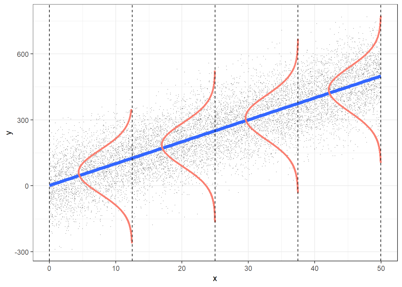
Since the mean of the error terms is 0, we expect the values of the response to equally distributed above and below the regression line.
5. The conditional expectation of the response
This theoretical formula may be a difficult to understand. It states that the (conditional) expected value of the response is linearly related with the input variables.
Example
Let’s consider the following simple LR in the CASchool example:
\(E\)(score|stratio) = a + m stratio
In this model, the average performance of students is associated with the ratio of students to teachers. Moreover, we expect a constant change in the student-teacher ratio will score to be linearly association changes linearly
in our example: \(E[\text{value}|\text{size}] = \beta_0 + \beta_1 \text{size}\)
Another way of viewing this assumption is that:
(for simplicity I’m omitting the subscript \(i\))
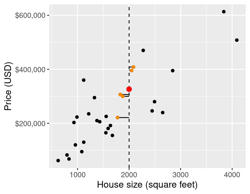
NOTE: This is not the only way to model the conditional expectation! If the true conditional expectation is not linear, other methods will be better to predict the response! For example: in DSCI100, you have used
kNN!
kNN vs LS
 |
 |
Images from Data Science: A First Introduction and Beyond Multiple Linear Regression (BMLR)
Estimation of the regression line
The true regression parameter are unknown! so we use data from a random sample to estimate them!!
options(repr.plot.width = 8, repr.plot.height = 5) # Adjust these numbers so the plot looks good in your desktop.

plot_value <- dat_s %>% ggplot(aes(BLDG_METRE, assess_val)) +
  geom_point() +
  xlab("building size (mts)") +
  ylab("assessment value ($/1000)") +
     geom_abline(intercept=145,slope=1.5, size=2, col = "grey")+
     geom_abline(intercept=500,slope=-1, size=2, col = "orange")+
     geom_abline(intercept=600,slope=-.5, size=2, col = "red")+
     geom_abline(intercept=10,slope=4, size=2, col = "green")+
     geom_abline(intercept=147,slope=1.9, size=2, col = "purple")+
  geom_smooth(method = lm, se = FALSE, color = "blue") +
  ggtitle("Random Sample and Estimated Linear Regression")
Error in dat_s %>% ggplot(aes(BLDG_METRE, assess_val)): could not find function "%>%"
Traceback:
plot_value
`geom_smooth()` using formula = 'y ~ x'
Which one is the best line??
Least Squares method minimizes the sum of the squares of the residuals!!
Note the residuals are the distances of each point to the estimated line
Check this application

1. LS in R
lm_s <- lm(assess_val~BLDG_METRE,data=dat_s)
tidy(lm_s)%>%mutate_if(is.numeric, round, 3)
| term | estimate | std.error | statistic | p.value |
|---|---|---|---|---|
| <chr> | <dbl> | <dbl> | <dbl> | <dbl> |
| (Intercept) | 90.769 | 9.793 | 9.268 | 0 |
| BLDG_METRE | 2.618 | 0.059 | 44.514 | 0 |
The formula in lm has the response variable before the ~ and the predictors after. In this case we have only one predictor (BLDG_METRE).
lm(assess_val~.,data=dat_s)uses all variables in the dataset, except the response, as predictors
2. Visualization of the LS line
Population points in grey and sample points in black
plot_value <- dat %>% ggplot(aes(BLDG_METRE, assess_val)) +
  geom_point(color = "grey") +
  xlab("building size (mts)") +
  ylab("assessed value ($/1000)") +
  geom_point(data = dat_s, aes(BLDG_METRE, assess_val), color = "black") +
  geom_smooth(method = lm, se = FALSE, color = "blue") +
  ggtitle("Random Sample and Estimated Linear Regression")
plot_value
`geom_smooth()` using formula = 'y ~ x'
3. The estimated slope
The estimated slope: \(\hat{\beta}_1=2.6\) measures the relationship between the assessment value and the size of a property
Interpretation:
Correct: An increase of 1 metre in size is associated with an increase of $2618 in the assessment value!
Wrong: The effect of 1 meter increase in the size of a property is a $2618 increase in the assessment value
Wrong: A 1 meter increase in the size of a property caused a $2618 increase in the assessed value
Important: We don’t know if the change in size caused the change in value and we can’t isolate the effect of size (holding other factors fixed) from all other factors in observational data
4. The estimated intercept
The estimated intercept: \(\hat{\beta}_0=90.8\) measures the expected assessment value for a property of size 0 mts.
We are not usually interested in this parameter
We can’t even think of it as the value of the land, it’s really an interpolated value of our model
Note that if the predictor is centered, \(X_{i}-\bar{X}\), then the intercept represents the value of a property of average size.
Important: Many statistical properties do not hold for models without intercept!
Parameter vs Estimator vs Estimate
3 important different concepts:
Course |
Population Parameter |
Estimator |
Estimate |
|---|---|---|---|
unknown quantity |
function of the random sample: random variable |
real number computed with data (non-random) |
|
STAT 201 |
mean = \(E[Y]\) |
sample mean = \(\bar{Y}\) |
499 |
STAT 301 |
slope = \(\beta_1\) |
estimator of the slope = \(\hat{\beta}_1 = \frac{\sum_{i=1}^n(X_i-\bar{X})(Y_i-\bar{Y})}{\sum_{i=1}^n(X_i-\bar{X})^2}\) |
2.6 |
Note: we use a “hat” over the coefficient to distinguish the estimator from the true coefficient
Note: usually \(\hat{\beta}_0\) and \(\hat{\beta}_1\) are used for both the estimates and the estimators, which can be confusing
Summary and Conclusions
Linear Regression Models provide a unifying framework to estimate and test the true relation between different type of variables and a continuous response
Linear Regression Models can also be used to predict the value of a continuous response (although it may not be the best predictive model)
We assume that the conditional expectation of the response is linearly related to the input variable and the line is the linear regression
Least Squares is one method to estimate the coefficients of a regression: it minimizes the sum of squares of the residuals
LS regression can be computed in R using the
lmfunctionUsing data from observational studies, we can not study any cause or effect between variables, only associations.
