Midterm 2 Info + Prep

Midterm 2 Information

TIMING/CONTENT

  • The second midterm is scheduled for in class on Friday Nov 20
  • It is 1 hour and 20 minutes
  • Your midterm will cover materials from Lectures 10 - 17

CHEATSHEET

  • You may bring (1) cheatsheet HAND WRITTEN with pen/pencil on one single sheet of paper (not typed, not photo copied, not printed, not written on an iPad)
  • Must be on 8.5 by 11 inch sheet of paper or smaller
  • You may write on both sides
  • I will confiscate cheatsheets that do not follow these rules
  • I do not care what is written on it

WRITING UTENSILS

  • Exam is hand written on paper, bring something to write with (preferably a pencil)

CALCULATORS

  • Non-programmable, non-graphing calculators only.
  • I will confiscate calculators that do not follow these rules

The final page of your midterm will also contain common distributions (download the sheet here)

Midterm 2 Preparation

Here are some selected problems that would serve as good practice for the midterm.

Finished these? Go back to the practice problems, checkpoints, and exercises/examples from lecture

Question 1

A residential building has an issue with toasters setting off the fire alarms frequently. Suppose that in a given building, there are an average of 2 fire alarms per week. Suppose the fire alarms are all independent. Let \(T\) be the time between successive alarms in days.

  1. What distribution does \(T\) follow? List the values of any parameters.

\(2 \frac{\text{alarms}}{\text{week}}= 2\frac{\text{alarms}}{\text{week}} * \frac{\text{1 week}}{\text{7 days}} = \frac{2}{7}\) alarms per day.

Thus,

\(T \sim {\mathrm{Exp}}(\lambda = 2/7)\) (or 0.286)

  1. What is the probability that the time between successive alarms will be exactly 2 days? Round your final answer to the nearest thousandth (i.e., 0.123).

Since this is a continuous distribution, \(P(X = a) = 0\).

  1. What is the probability that the time between successive alarms is more than 4 days? Round your final answer to the nearest thousandth (i.e., 0.123).

\[ \begin{aligned} P(T > 4) &= \int_{4}^{\infty} \frac{2}{7}e^{-2/7t}dt\\ &= \frac{2}{7}\frac{-7}{2} e^{-2/7t} \big|_{t = 4}^{t = \infty}\\ &= e^{-2/7(4)}\\ &= 0.319 \end{aligned} \]

Question 2

Let \(X\) have the PMF \(\mathbb{P}(X = k) = \frac{1}{6} I_{\{1,2,3,4,5,6\}}(x)\).

  1. Find the PMF of \(Y = min(X, 7 - X)\).

First, consider the possible values of \(Y\) by computing \(\min(X, 7-X)\) for each value of \(X\):

\(X\) \(7-X\) \(Y = \min(X, 7-X)\)
1 6 1
2 5 2
3 4 3
4 3 3
5 2 2
6 1 1

So \(Y\) takes values in \(\{1, 2, 3\}\).

Then, for each value of \(Y\) solve for the probability.

Each value of \(X\) has probability \(\frac{1}{6}\), so:

\[P(Y = 1) = P(X=1) + P(X=6) = \frac{2}{6} = \frac{1}{3}\]

\[P(Y = 2) = P(X=2) + P(X=5) = \frac{2}{6} = \frac{1}{3}\]

\[P(Y = 3) = P(X=3) + P(X=4) = \frac{2}{6} = \frac{1}{3}\]

Thus, \(P(Y = y) = \frac{1}{3}I_{\{1,2,3\}}(y)\)

  1. Find the CDF of \(Y\).

From a), the PDF is \(P(Y = y) = \frac{1}{3}I_{\{1,2,3\}}(y)\).

Thus, the CDF is:

$$ F_X(x) = P(Y y) = \[\begin{cases} 0 & \text{ for } x < 1\\ \frac{1}{3} &\text{ for } 1 \le x < 2\\ \frac{2}{3} &\text{ for } 2 \le x < 3\\ 1 &\text{ for } x \ge 3\\ \end{cases}\]

$$

Question 3

Let \(X \sim {\mathrm{Exp}}(1)\).

  1. Find the PDF of \(Y = \sqrt{X}\) using the Jacobian method.

First, we know that \(f_X(x) = e^{-x}I_{[0, \infty)}(x)\).

Then we have \(y = h(x) = \sqrt{x}\), so \(x = h^{-1}(y) = y^2\), valid for \(y \ge 0\).

Since the transformation is monotonically increasing and differentiable, we can use the Jacobian method.

\[\frac{d}{dy}h^{-1}(y) = \frac{d}{dy}y^2 = 2y\]

Now we can plug into the formula:

\[f_Y(y) = f_X(h^{-1}(y))\left|\frac{dh^{-1}(y)}{dy}\right| = e^{-y^2}2y I_{[0, \infty}(y)\]

  1. Find the PDF of \(Y = \sqrt{X}\) using the Distribution method.

The CDF of \(X\) is

\[ F_X(x) = \int_{0}^xe^{t}dt = (1 - e^{-x})I_{[0, \infty)}(x) \] Thus,

\[ \begin{aligned} F_Y(y) &= \mathbb{P}(Y \le y)) \\ &= \mathbb{P}(\sqrt(X) \le y)\\ &= \mathbb{P}(X \le y^2) \\ &= (1 - e^{-(y^2)})I_{[0, \infty)}(y^2)\\ &= (1 - e^{-y^2})I_{[0, \infty)}(y)\\ \end{aligned} \]

Then, the PDF is:

\[ \begin{aligned} f_Y(y) &= \frac{d}{dy}F_Y(y) \\ &= -e^{-y^2}(-2y)I_{[0, \infty]}(y)\\ &= 2e^{-y^2}I_{[0, \infty)}(y) \end{aligned} \]

Question 4

Let \(X\) and \(Y\) be independent \({\mathrm{Exp}}(\lambda)\) random variables,. Find the PDF of \(U = X + Y\) using the convolution method.

Hint: be careful with the limits of integration. Recall that if \(Z\sim {\mathrm{Exp}}(\theta)\), then \(f_Z(z) = \theta e^{-\theta z}I_{(0,\infty)}(z)\).

Using the convolution method, we have that for \(u < 0\), \(f_U(u) = 0\), and for \(u > 0\), we have that \[\begin{aligned} f_U(u) &= \int_{-\infty}^\infty f_X(x) f_Y(u - x) \mathsf{d}x \\ &= \int_0^u \lambda e^{-\lambda x} \lambda e^{-\lambda (u - x)} \mathsf{d}x \\ &= \lambda^2 e^{-\lambda u} \int_0^u \mathsf{d}x \\ &= \lambda^2 u e^{-\lambda u}. \end{aligned}\] Therefore, \(U\) has PDF \(f_U(u) = \lambda^2 u e^{-\lambda u}I_{(0,\infty)}(u)\), so \(U \sim {\mathrm{Gam}}(2, \lambda)\).

Question 5

Let \(X\) be a discrete random variable with probability function

\[ p_X(x) = \begin{cases} 2^{-x} & x = 1, 2, 3, ... \\ 0 &\text{otherwise} \end{cases} \]

Let \(Z = X - 1\).

  1. Compute the probability mass function of \(Z\).

\[ \begin{aligned} p_Y(y) &= \sum_{x: g(x) = z} p_X(x)\\ &= \sum_{x: x-1 = z} p_X(x)\\ &= p_{X}(z+1)\\ &= 2^{-(z+1)}I_{\{0,1,2,...\}}(z) \end{aligned} \]

  1. Name the distribution of \(Z\) that you found in part (a), and identify its parameters.

\[ \begin{aligned} 2^{-(z+1)}I_{\{0,1,2,...\}}(z) &= 2^{-z}2^{-1}I_{\{0,1,2,...\}}(z)\\ &= (1/2)^z(1/2)I_{\{0,1,2,...\}}(z)\\ &= (1 - 1/2)^z(1/2))I_{\{0,1,2,...\}}(z) \end{aligned} \]

Thus, \(Z \sim {\mathrm{Geom}}(1/2)\)

Question 6

  1. Let \[f_{X,Y}(x,y) = \frac{1}{24}(x+2y)\, I_{(0,2)}(x)\, I_{(0,3)}(y).\] Find \(\mathbb{P}(Y < 2X)\).

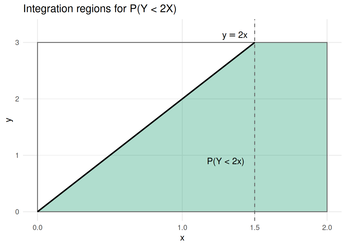
There are many possible ways to solve for this probability. We can visualize the integration area first, to help us decide how to solve this problem:

Method 1: Taking a complement

It’s easier to integrate the white area (\(\mathbb{P}(Y \ge 2X)\)) directly.

\[ \begin{aligned} \mathbb{P}(Y < 2X) &= 1 - \mathbb{P}(Y \ge 2X)\\ &= 1 -\int_0^{1.5}\int_{2x}^3 \frac{1}{24}(x + 2y)\,dy\,dx \\ &= 1 - \frac{1}{24}\int_0^{1.5} \left(xy + y^2\right)\Big|_{y = 2x}^{y = 3}dx\\ &= 1- \frac{1}{24}\int_0^{1.5} \left(3x + 9 - 6x^2\right)dx\\ &= 1-\frac{1}{24}\left(\frac{3x^2}{2} + 9x - 2x^3\right)\Big|_{x=0}^{x=1.5}\\ &= 1-\frac{1}{24}\left(3.375 + 13.5 - 6.75\right) \\ &=1- \frac{27}{64}\\ &= \frac{37}{64} \end{aligned} \]

So \(\mathbb{P}(Y < 2X) = 1 - \frac{27}{64} = \frac{37}{64} \approx 0.578\).

NOTE: you can also integrate over \(X\) first. As \(y/2 \le 1.5 < 2\), the upper limit of \(x\) never exceeds its support:

\[ \begin{aligned} \mathbb{P}(Y < 2X) &= 1 - \mathbb{P}(Y \ge 2X)\\ &= 1 -\int_0^{3}\int_{0}^{y/2} \frac{1}{24}(x + 2y)\,dx\,dy \\ &= 1 - \frac{1}{24}\int_0^{3} \left(\frac{x^2}{2} + 2xy\right)\Big|_{x = 0}^{x = y/2}dy\\ &= 1- \frac{1}{24}\int_0^{3} \left(\frac{y^2}{8} + y^2\right)dy\\ &= 1- \frac{1}{24}\int_0^{3} \frac{9y^2}{8}\,dy\\ &= 1-\frac{1}{24}\left(\frac{3y^3}{8}\right)\Big|_{y=0}^{y=3}\\ &= 1-\frac{1}{24}\left(\frac{81}{8}\right) \\ &=1- \frac{27}{64}\\ &= \frac{37}{64} \end{aligned} \]

Method 2: Splitting into two regions

We can still solve for this probability directly, but you’d have to split it into two integrals.

\[ \begin{aligned} \mathbb{P}(Y < 2X) &= \int_0^{1.5}\int_{0}^{2x} \frac{1}{24}(x + 2y)\,dy\,dx + \int_{1.5}^{2}\int_{0}^{3} \frac{1}{24}(x + 2y)\,dy\,dx\\ &= \frac{1}{24}\int_0^{1.5} 6x^2\,dx + \frac{1}{24}\int_{1.5}^{2}(3x+9)\,dx\\ &= \frac{1}{24}(6.75) + \frac{1}{24}(7.125)\\ &= \frac{37}{64} \approx 0.578 \end{aligned} \]

Note: for \(x \in (0, 1.5)\) the upper limit of \(y\) is \(2x\), but for \(x \in (1.5, 2)\) we have \(2x > 3\), so \(Y < 2X\) holds for every \(y\) in its support and the upper limit is 3. Using \(y \in (0, 2x)\) all the way to \(x = 2\) would integrate over values of \(y\) outside the support.

  1. Find the marginal PDF \(f_X(x)\).

\[ \begin{aligned} f_X(x) &= \int f_{X,Y}(x,y)dy\\ &= \int_0^3\frac{1}{24}(x+2y)\, I_{(0,2)}(x)dy\\ &= \frac{1}{24}(xy + y^2)|_{y = 0}^{y = 3}I_{(0,2)}(x)\\ &= \frac{1}{8}(x + 3)I_{(0,2)}(x)\\ \end{aligned} \]

  1. Find the marginal CDF \(F_X(x)\).

The CDF is:

\[ F_X(x) = \begin{cases} 0 & \text{ for } x \le 0\\ \int_0^x \frac{1}{8}(t+3)dt = \frac{1}{16}(x^2 + 6x) &\text{ for } 0 < x < 2\\ 1 &\text{ for } x \ge 2\\ \end{cases} \]

Question 7

Let \(X \sim {\mathrm{Exp}}(2)\).

  1. What is \(\mathbb{E}[X^2]\)?

One way to solve this is with kernel matching: \[ \begin{aligned} \mathbb{E}\left[X^2\right] &= \int x^2f_X(x)dx\\ &= \int_0^{\infty} x^2 2e^{-2x}dx\\ &= 2\int_0^{\infty} x^{3-1}e^{-2x}dx\\ &= 2\frac{\Gamma(3)}{2^3}\int_0^{\infty} \frac{2^3}{\Gamma(3)} x^{3-1}e^{-2x}dx\\ &= 2\frac{2}{2^3}\\ &= \frac{1}{2} \end{aligned} \]

  1. Let \(Y = 3X^2 + 2\). What is \(\mathbb{E}[Y]\)?

\[ \begin{aligned} \mathbb{E}[Y] &= \mathbb{E}[3X^2+2] \\ &= 3\mathbb{E}[X^2] + 2 \\ &= 3\frac{1}{2} + 2\\ &= \frac{7}{2} \end{aligned} \]

Question 8

Suppose \(X\) and \(Y\) have joint PMF:

\(Y=1\) \(Y=2\)
\(X=0\) 1/12 2/12
\(X=1\) 3/12 1/12
\(X=2\) 1/12 4/12

and 0 otherwise.

  1. What is \(\mathbb{E}[X]\)?

We first need the marginal PMF of X: \[ P_X(X=x) = \begin{cases} \frac{3}{12} & x = 0\\ \frac{4}{12} & x = 1\\ \frac{5}{12} & x = 2 \\ 0 & \text{otherwise} \end{cases} \]

Then, the expected value is:

\[ \begin{aligned} \mathbb{E}[X] = \frac{3}{12}(0) + \frac{4}{12}(1) + \frac{5}{12}(2) = \frac{7}{6} \end{aligned} \]

  1. What is \(\mathbb{E}[(XY)^2]\)?

\[ \begin{aligned} \mathbb{E}[XY] &= \sum_x\sum_y (xy)^2 p_{XY}(x,y)\\ &= \frac{1}{12}(0 \cdot1)^2 + \frac{2}{12}(0 \cdot 2)^2 + \frac{3}{12}(1 \cdot 1)^2 + \frac{1}{12}(1\cdot2)^2\\ & \hspace{1cm}+ \frac{1}{12}(2 \cdot 1)^2 + \frac{4}{12}(2 \cdot 1)^2\\ &= \frac{25}{4} \end{aligned} \]

Question 9

Let \(X\) and \(Y\) have joint density \(f_{X,Y}(x,y) = c\,(x + 2y)\,I_{(0, 1)}(x)I_{(x, 1)}(y)\).

  1. Find the constant \(c\) that makes this a valid density.

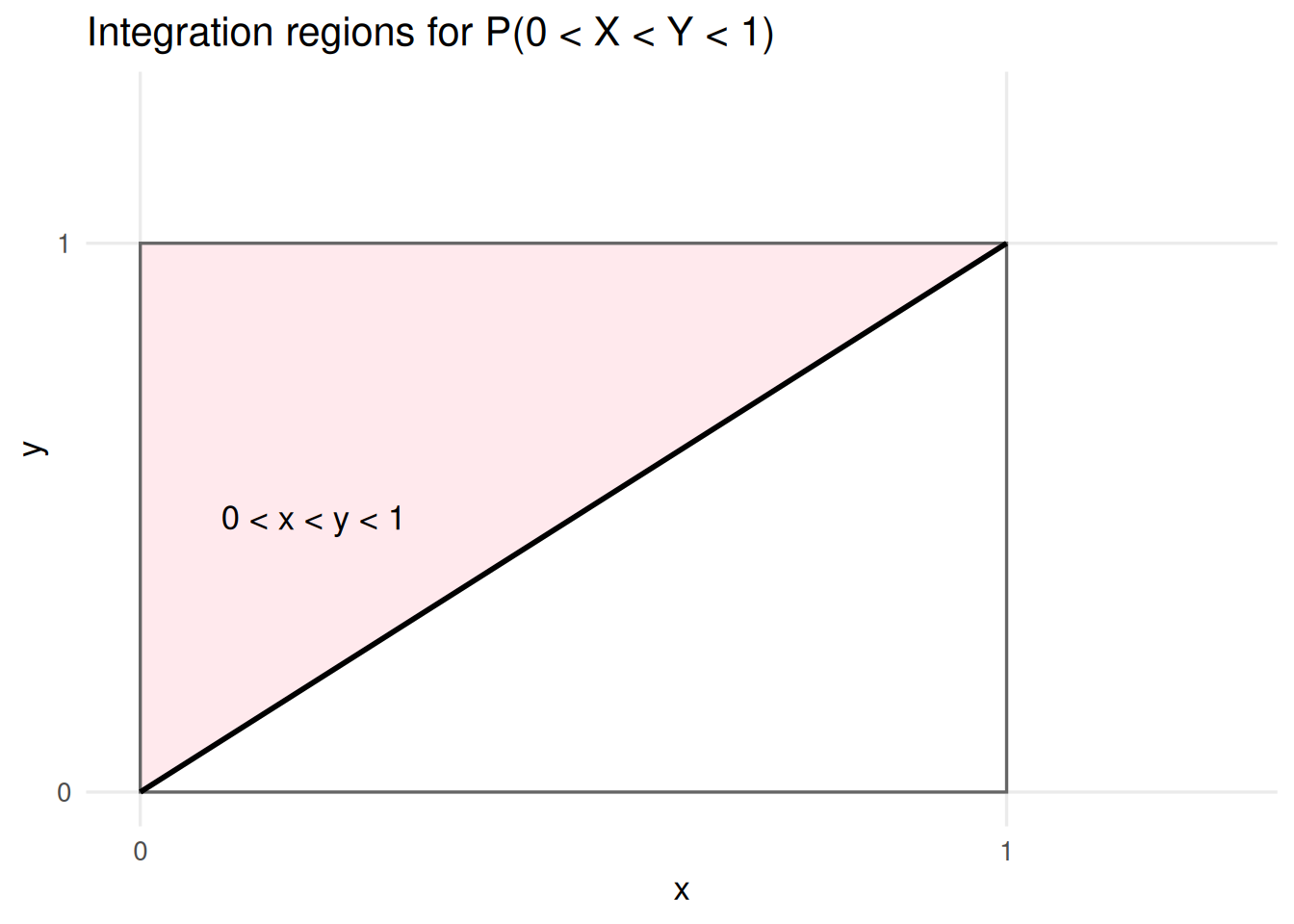
The density must integrate to 1 over the triangle \(0 < x < y < 1\).
\[ \begin{aligned} \int_0^1 \int_x^1 (x + 2y)\,dy\,dx &= \int_0^1 \left( xy + y^2 \Big|_{y=x}^{y=1} \right) dx \\ &= \int_0^1 \left( x(1-x) + (1 - x^2) \right) dx \\ &= \int_0^1 \left( 1 + x - 2x^2 \right) dx \\ &= 1 + \frac{1}{2} - \frac{2}{3} = \frac{5}{6} \end{aligned} \]

so \(c = \dfrac{6}{5}\).

(NOTE: you can also integrate over \(X\) first. How will the bounds change?).

  1. Compute the conditional density \(f_{Y \ \vert\ X}(y \ \vert\ x)\) for \(f_X(x) > 0\).

The marginal pdf of \(X\) is

\[ \begin{aligned} f_X(x) &= \int_x^1 \frac{6}{5}(x + 2y)\,dy \; I_{(0,1)}(x) \\ &= \frac{6}{5}\left( 1 + x - 2x^2 \right) I_{(0,1)}(x) \\ &= \frac{6}{5}(1-x)(1+2x)\, I_{(0,1)}(x) \end{aligned} \]

Then

\[ \begin{aligned} f_{Y \ \vert\ X}(y \ \vert\ x) &= \frac{\frac{6}{5}(x + 2y)\,I_{(0, 1)}(x)I_{(x, 1)}(y)}{\frac{6}{5}(1-x)(1+2x)\, I_{(0,1)}(x)} \\ &= \frac{x + 2y}{(1-x)(1+2x)}\,I_{(x, 1)}(y) \end{aligned} \]