viewof answer6_1_1_part1 = Inputs.radio(["variance", "proportion", "standard deviation", "mean"], {label: "Parameter: "})6 Module 6: Simulation-based hypothesis testing
Learning objectives
Give an example of a question you could answer with a hypothesis test.
Differentiate composite vs. simple hypotheses.
Given an inferential question, formulate null and alternative hypotheses to be used in a hypothesis test.
Identify the steps and components of a basic hypothesis test (“there is only one hypothesis test”).
Write computer scripts to perform hypothesis testing via simulation, randomization and bootstrapping approaches, as well as interpret the output.
Describe the relationship between confidence intervals and hypothesis testing.
Discuss the potential limitations of this simulation approach to hypothesis testing.
Introduction
So far in the course, we have focused our attention on estimation, where we are interested in unknown parameters of a specific population. Our objective was to estimate these unknown parameters as accurately as possible. We discussed two types of estimators:
Point estimators: just a number we calculate from our sample (i.e., a statistic).
Interval estimators: a range of plausible values for a parameter which accounts for the uncertainty associated with the estimation process (i.e., confidence intervals).
However, in many situations, we are not mainly interested in the precise value of the parameter. Instead, we need to assess specific claims or assumptions about the population, which can lead to different conclusions or decisions. To better understand this, let us consider the Vancouver Beaches problems introduced in the example below.
Example 6.1 During the summer, Vancouver’s beaches get pretty busy. To ensure everybody’s safety, the city of Vancouver monitors if the beaches’ waters are safe for swimming. If the average number of E. coli per 100mL is 400 or less, the city considers the beach proper for swimming. Otherwise, the city of Vancouver releases a public statement to warn people that they should not swim on the beach. How should the city proceed?
□
In Example 6.1 above, we have two competing statements: (1) the beach is safe for swimming (i.e., the average number of E. Coli per 100mL is 400 or less); and (2) the beach is unsafe for swimming (i.e., the average number of E. Coli per 100mL is higher than 400). The city’s responsibility is to determine which of these statements holds true, and to communicate the findings clearly to the public. Their primary objective is not to obtain an exact measurement of the average E. Coli level but rather to ascertain whether it falls at or below the threshold of 400. The specific numerical values, such as whether the average is 75 or 100 E. Coli per 100 milliliters, are less important; what matters is the city’s ability to confidently and reliably identify which statement regarding the beach’s safety is accurate.
Statistical hypothesis testing provides a structured framework for evaluating the strength of evidence contained in a dataset against specific claims or assumptions regarding a broader population. In this chapter, we will delve into the methodology of conducting statistical tests designed to assess various hypotheses related to population characteristics. We’ll explore the principles behind these tests, the types of hypotheses that can be evaluated, and the procedures for drawing conclusions based on the analysis of the data. Through this discussion, we aim to equip you with the necessary tools to statistically assess the validity of claims about a population.
6.1 Statistical Hypotheses: Null vs Alternative
Let us start by defining what a hypothesis is.
Definition 6.1 (Statistical Hypothesis) A statement about one or more populations.
Although the Definition 6.1 is quite broad, a hypothesis usually involves a statement about population parameters. Therefore, in this book, we will restrict our attention to hypotheses that are statements about parameters of population(s).
In statistical hypothesis testing, we always have two competing and complementary hypotheses: the null hypothesis (denoted as H_0) and the alternative hypothesis (denoted as H_A or H_1). The null hypothesis represents a default or status quo assumption about the population parameter, often reflecting a lack of effect or no difference. Conversely, the alternative hypothesis represents the claim of effect for which we are trying to find evidence. The goal of hypothesis testing is to assess whether the sample data provides sufficient evidence to reject the null hypothesis in favor of the alternative hypothesis.
6.1.1 Hypotheses involving one population
When we are testing only one parameter of a given population, we usually have a threshold of interest, which we call \mu_0 (for the mean; read mu naught) and p_0 (for the proportion; read p naught), and the null hypothesis will have the following form:
H_0: \mu = \mu_0
and the alternative hypothesis will have one (and only one) of the following three forms:
- H_A: \mu < \mu_0
- H_A: \mu > \mu_0
- H_A: \mu \neq \mu_0
Naturally, in the case above, we are testing the mean. But we could be testing any other parameter. For example, for proportion, we would replace \mu with p: H_0: p = p_0. Let’s see a few examples.
Example 6.2 A pharmaceutical company has developed a new flu vaccine and wants to determine if it’s more effective than the standard flu vaccine currently in use. The standard vaccine is known to be effective in preventing the flu in 60% of the population who receive it. The company conducts a clinical trial where a random sample of individuals receives the new vaccine. Is the new vaccine more effective than the standard vaccine? The hypotheses are:
H_0: p = 0.60 \quad\quad\text{vs}\quad\quad H_A: p > 0.60
□
Frequently, as in the example above, we can unambiguously identify the null hypothesis. But sometimes, it depends on the problem. See the following two examples.
Example 6.3 Heart disease is one of the leading causes of death worldwide, and high cholesterol is a significant risk factor. Medical guidelines recommend that the average level of low-density lipoprotein (LDL), often referred to as “bad” cholesterol, should be below 100 mg/dL to help minimize the risk of heart disease.
In Canada, the government is considering a new community health initiative aimed at reducing heart disease deaths. This initiative would cost approximately $1.23 billion annually. The Official Opposition Party is urging the government to avoid unnecessary expenditures. As a compromise, the government has stated that it would drop the project if there is strong evidence showing that the Canadian population has a lower risk of heart disease due to low cholesterol levels.
In this case, we have H_0: \mu = 100\text{mg/dL}\quad\quad\text{vs}\quad\quad H_A: \mu < 100\text{mg/dL} Therefore, our hypotheses are statements about the mean LDL cholesterol in the Canadian population. Also, note that the government is demanding evidence to believe Canadians are low risk (as opposed to requiring evidence that Canadians are high risk). For this reason, we have the “low risk” case in the alternative hypothesis.
Alternatively, if the government had said that they would only proceed with the program if there were strong evidence that Canadians are at high risk of heart disease, then we would formulate the hypotheses as:
H_0: \mu = 100\text{mg/dL}\quad\quad\text{vs}\quad\quad H_A: \mu > 100\text{mg/dL}
Note how the burden of evidence changes (but also the boundary value, in the former formulation 100 mg/dL was considered high risk, while in the latter formulation it is considered low risk).
□
Example 6.4 Going back to the Vancouver Beaches example (Example 6.1). If the city council works under the assumption that the beaches are usually improper for swimming (status quo), they will require evidence that the beaches are safe for swimming. In this case, H_0: \mu = 400\quad\quad\text{vs}\quad\quad H_A: \mu < 400
Alternatively, the city council could claim that it is very expensive to close the beaches, and they want to do it only if they have evidence that the beaches are not safe for swimming. Then:
H_0: \mu = 400\quad\quad\text{vs}\quad\quad H_A: \mu > 400
Again, note how the burden of evidence changes (but also the boundary value, in the former formulation 400 E. Coli per 100 mL is considered unsafe, whereas in the second formulation it is considered safe).
□
In statistical hypothesis testing, we begin by assuming that one of two hypotheses, H_0 (the null hypothesis) or H_A (the alternative hypothesis), is true. However, we do not know which one, and our goal is to determine that. A common question that arises is: what if neither hypothesis is true?
For example, let’s consider the situation presented by Example 6.2. The hypotheses are defined as follows: H_0: p = 0.6 versus H_A: p > 0.6. But what if the vaccine actually has a negative effect? This raises the possibility that, after receiving the vaccine, p could be less than 0.6. If we believe this scenario is a real possibility, we could redefine the null hypothesis to be H_0: p \leq 0.6 versus H_A: p > 0.6. This way, we encompass all possible outcomes within our two hypotheses.
Fortunately, for the tests discussed in this book, this adjustment does not affect the results of the hypothesis test. Therefore, the procedure we will follow remains the same whether we use H_0: p = 0.6 or H_0: p \leq 0.6. For this reason, in this book, we will always express the null hypothesis using the equal sign as follows: H_0: p = p_0.
6.1.2 Hypotheses involving two populations
When comparing two populations, we are often interested in examining the values of their parameters. Typically, the null hypothesis is stated as:
H_0: \mu_1 - \mu_2 = \Delta_0 The alternative hypothesis could take one of the following forms:
- H_A: \mu_1-\mu_2 < \Delta_0
- H_A: \mu_1-\mu_2 > \Delta_0
- H_A: \mu_1-\mu_2 \neq \Delta_0
Let’s see some examples.
Example 6.5 Tech Solutions, a software company, is testing two different versions of their website’s landing page. They want to know if one version leads to a higher proportion of visitors signing up for a free trial. They randomly assign website visitors to either version A or version B. They track the number of visitors who sign up for a free trial on each version. In this case, the hypotheses are: H_0: p_1-p_2=0 \quad\quad \text{ vs } \quad\quad H_A: p_1-p_2\neq0 where p_1 and p_2 are the proportion of sign-ups for versions A and B, respectively. Or, in another words:
H_0: There is no difference in the proportion of visitors who sign up for a free trial between the two landing page versions.
H_A: There is a difference in the proportion of visitors who sign up for a free trial between the two landing page versions.
Note that in this case, we used \Delta_0 = 0.
□
Example 6.6 Green Thumb Gardens wants to test two different fertilizer types to see which promotes better plant growth. They are specifically interested in the average height of tomato plants after a certain period. They take a batch of young tomato plants and randomly assign them to two groups. Group A receives Fertilizer GrowFast, and Group B receives Fertilizer BloomBoost. After six weeks, they measure the height of each plant in centimetres. They want to determine if there is a difference in the average height of tomato plants between the two fertilizer groups.
H_0: \mu_1-\mu_2=0 \quad\quad \text{ vs } \quad\quad H_A: \mu_1-\mu_2\neq0 where \mu_1 is the mean height of plants using Fertilizer GrowFast, and \mu_2 is the mean height of plants using Fertilizer BloomBoost. Or, in words:
H_0: There is no difference in the average height of tomato plants between the two fertilizer groups.
H_A: There is a difference in the average height of tomato plants between the two fertilizer groups.
□
With a clear understanding of how to define statistical hypotheses, we are now equipped to delve into the mechanics of hypothesis testing.
6.1.3 Exercises
Exercise 6.1 A school district is considering implementing a new reading program to improve literacy rates among its students. The current average reading score on a standardized test is 75 out of 100. The district will only adopt the new program if there is strong evidence that the new program increases the average reading score.
(a) Which of the following parameters is more relevant in this case?
#| edit: false
#| echo: false
#| output: true
#| input:
#|   - answer6_1_1_part1

# Checks your answer for Exercise 6.1.1

if (!is.na(answer6_1_1_part1)){
  if (answer6_1_1_part1 == "mean"){
    cat("You've got it! Nice job!\U1F389")
  }
  else{
    cat("Oopsy, try again! You can do this! \U1F4AA")
  }
}
(b) How would you formulate the null hypothesis?
(Here \theta represents the parameter of interest.)
- H_0: \theta = 75\%
- H_0: \theta > 75
- H_0: \theta = 75
- H_0: \theta < 75
- H_0: \theta \neq 75
#| edit: false
#| echo: false
#| output: true
#| input:
#|   - answer6_1_1_part2

# Checks your answer for Exercise 6.1.1 part 2

if (!is.na(answer6_1_1_part2)){
  if (answer6_1_1_part2 == "(C)"){
    cat("You've got it! Nice job!\U1F389")
  }
  else{
    cat("Oopsy, try again! You can do this! \U1F4AA")
  }
}
(c) How would you formulate the alternative hypothesis?
(Here \theta represents the parameter of interest.)
- H_A: \theta = 75\%
- H_A: \theta > 75
- H_A: \theta = 75
- H_A: \theta < 75
- H_A: \theta \neq 75
#| edit: false
#| echo: false
#| output: true
#| input:
#|   - answer6_1_1_part3

# Checks your answer for Exercise 6.1.1 part 3

if (!is.na(answer6_1_1_part3)){
  if (answer6_1_1_part3 == "(B)"){
    cat("You've got it! Nice job!\U1F389")
  }
  else{
    cat("Oopsy, try again! You can do this! \U1F4AA")
  }
}
Exercise 6.2 A smartphone manufacturer claims that 90\% of their customers are satisfied with their product. A consumer advocacy group wants to test this claim and will challenge it if there is strong evidence that the true satisfaction rate is different from $90$%.
(a) Which of the following parameters is more relevant in this case?
#| edit: false
#| echo: false
#| output: true
#| input:
#|   - answer6_1_2_part1

# Checks your answer for Exercise 6.1.2

if (!is.na(answer6_1_2_part1)){
  if (answer6_1_2_part1 == "proportion"){
    cat("You've got it! Nice job!\U1F389")
  }
  else{
    cat("Oopsy, try again! You can do this! \U1F4AA")
  }
}
(b) How would you formulate the null hypothesis?
(Here \theta represents the parameter of interest.)
- H_0: \theta = 90\%
- H_0: \theta > 90\%
- H_0: \theta < 90\%
- H_0: \theta \neq 90\%
#| edit: false
#| echo: false
#| output: true
#| input:
#|   - answer6_1_2_part2

# Checks your answer for Exercise 6.1.1 part 2

if (!is.na(answer6_1_2_part2)){
  if (answer6_1_2_part2 == "(A)"){
    cat("You've got it! Nice job!\U1F389")
  }
  else{
    cat("Oopsy, try again! You can do this! \U1F4AA")
  }
}
(c) How would you formulate the alternative hypothesis?
(Here \theta represents the parameter of interest.)
- H_0: \theta = 90\%
- H_0: \theta > 90\%
- H_0: \theta < 90\%
- H_0: \theta \neq 90\%
#| edit: false
#| echo: false
#| output: true
#| input:
#|   - answer6_1_2_part3

# Checks your answer for Exercise 6.1.1 part 3

if (!is.na(answer6_1_2_part3)){
  if (answer6_1_2_part3 == "(D)"){
    cat("You've got it! Nice job!\U1F389")
  }
  else{
    cat("Oopsy, try again! You can do this! \U1F4AA")
  }
}
6.2 The idea of hypothesis testing
Testing hypotheses is similar to being a detective. Detectives do not witness crimes directly; instead, they determine who committed a crime based on the aftermath. This process typically involves considering various scenarios (or hypotheses) and checking whether the evidence collected supports or contradicts them. Importantly, detectives look for evidence that contradicts the “innocent” hypothesis. This is similar to the principle of “innocent until proven guilty” (in statistics, we assume the null hypothesis is true until we find sufficient evidence to reject it).
How does this relate to statistics?
The null hypothesis, denoted as H_0, is either true or false, but we cannot observe it directly—similar to how a detective does not witness the crime being committed. We are unable to observe it directly because we do not have access to the entire population, which means we do not know the true value of the parameter.
However, the null hypothesis, H_0, implies a specific sampling distribution for some statistics (the aftermath). We can then take a sample and contrast the value of the statistic against the sampling distribution if H_0 were true.
Let’s revisit Example 6.2. Suppose we take a sample of 50 patients. Since we are testing the population proportion, we can use the sample proportion \hat{p} to gain insights about the population mean. If the null hypothesis were true, we know from the Central Limit Theorem (CLT) that \hat{p} \sim N\left(0.6, \sqrt{\frac{0.6 \times 0.4}{50}}\right). If we used different values for p_0 in H_0, the sampling distribution would change accordingly. See the plot below.
The plot above illustrates the sampling distribution of the sample proportion, assuming the null hypothesis is true. As you adjust the value of p_0, the distribution shifts accordingly. Note, however, that if p_0 happens to be the same as p, then the null model coincides with the sampling distribution. But of course, in this case, the null hypothesis would be actually true.
Finally, we can collect the data (the evidence), calculate the sample proportion \hat{p}, and compare it to the sampling distribution under the null hypothesis H_0. If the calculated value of the statistic is plausible under H_0, we do not have enough evidence to reject the hypothesis. For instance, in the case of Example 6.2, where p_0 = 0.6, suppose that after collecting our sample, of size 50 we calculate a sample proportion of \hat{p} = 0.95. The sampling distribution and the statistic are shown in Figure 6.2.
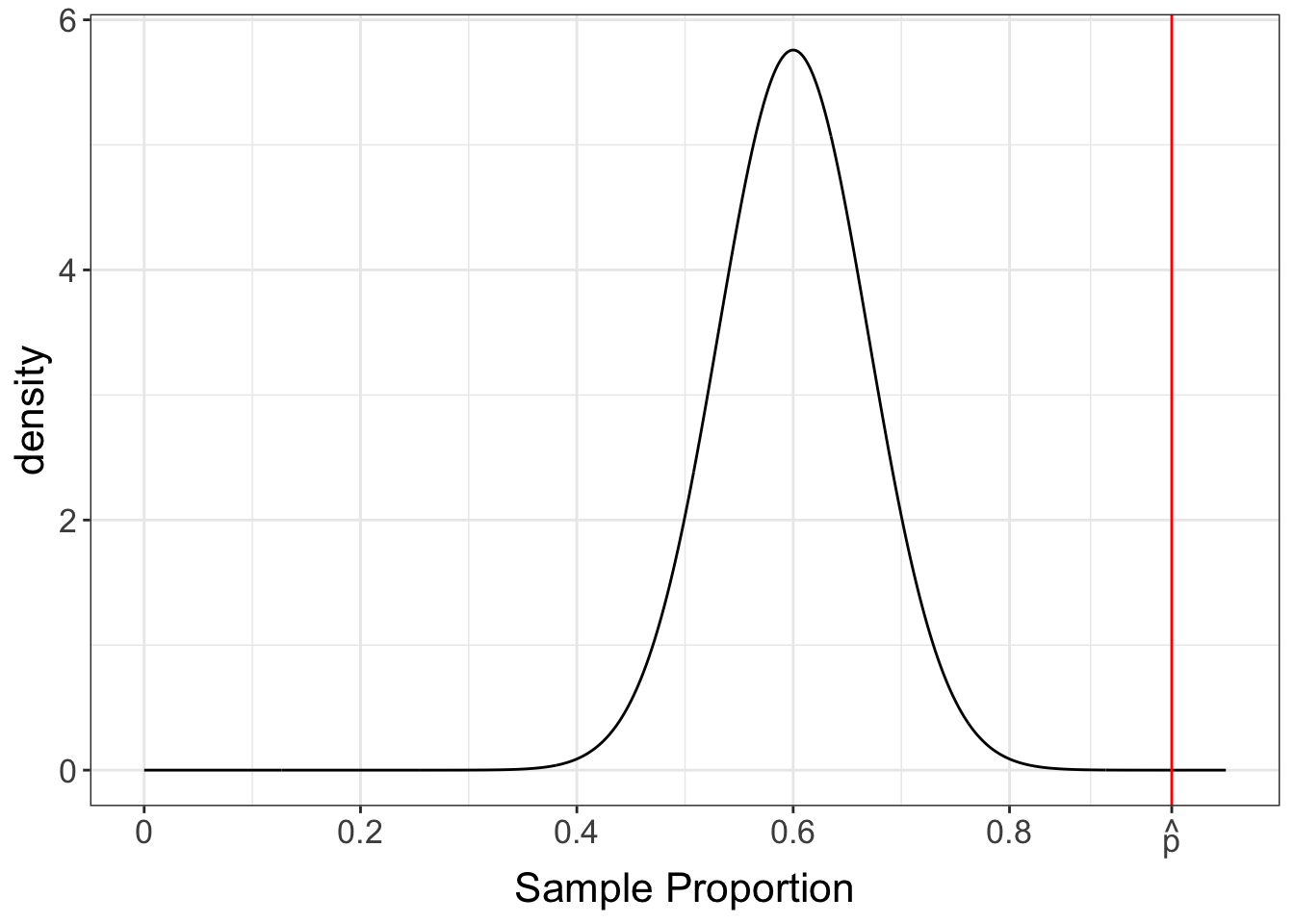
As noted by Figure 6.2, the observed value \hat{p} = 0.95 is VERY unlikely to occur if the null hypothesis H_0 is true. Therefore, we have two possibilities: either we were simply unlucky and ended up with an unusual sample, or the null hypothesis H_0 is false. This suggests that the distribution shown in Figure 6.2 does not accurately represent the true sampling distribution of \hat{p}. This situation is akin to a detective finding the murder weapon with the suspect’s fingerprint on it. While this evidence strongly suggests the suspect’s guilt, it does not conclusively prove it.
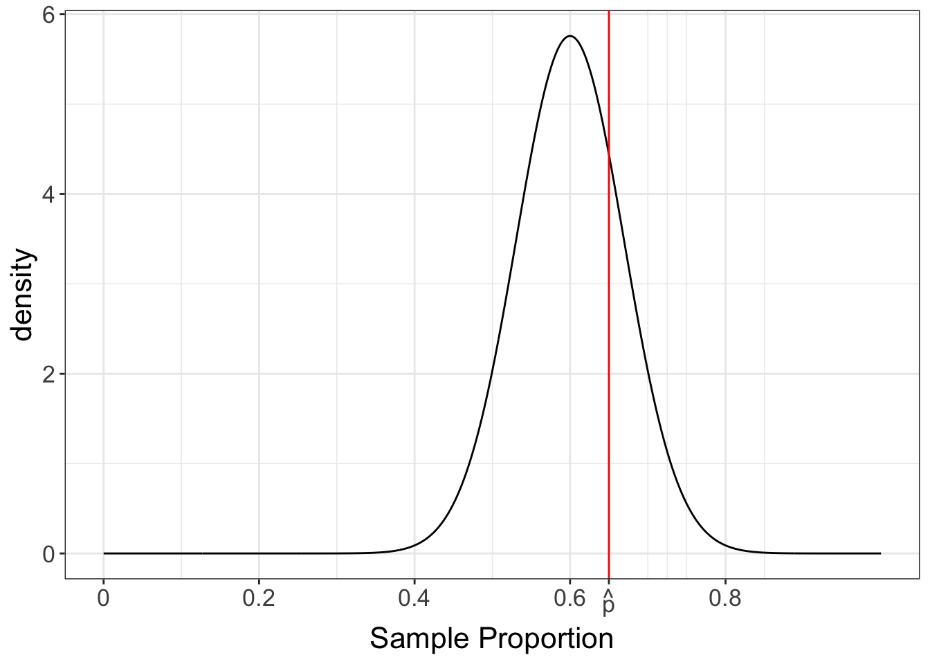
Let’s consider an alternative scenario where we collect a sample of size 50, and the sample proportion is \hat{p} = 0.65. In this case, it wouldn’t be surprising to observe this \hat{p} value if the null hypothesis H_0 were true (see Figure 6.3). Therefore, the observed value of \hat{p} does not contradict the hypothesis H_0, indicating that the evidence against H_0 is weak. However, this does not imply that H_0 is true; it simply means that we lack strong evidence to reject it. It’s similar to a detective who cannot find conclusive evidence against a suspect; this absence of evidence does not prove the suspect’s innocence. In other words, the absence of evidence of guilt is not the same as evidence of innocence.
The core idea of hypothesis testing involves comparing our data to what we’d expect under the null hypothesis. But how do we actually do that in practice? The next section will provide a detailed, step-by-step guide to the hypothesis testing procedure, equipping you with the tools to apply these concepts to real-world problems.
6.3 The steps in hypothesis testing
In this book, we will discuss different strategies for hypothesis testing as well as many different hypothesis tests. However, no matter the strategy and the test, we will always be guided by five steps:
- Step 1: Formulate the Hypotheses
- Step 2: Define the desired significance level
- Step 3: Define an appropriate test statistic
- Step 4: Identify the null model
- Step 5: Calculate the p-value
In the following sections, we will discuss each of these steps in detail.
6.3.1 Step 1: Formulate the Hypotheses
In this step, it is essential to clearly define the null hypothesis (H_0) and the alternative hypothesis (H_A). Often, this step in the research process does not receive adequate attention, but formulating these hypotheses is crucial. They guide our statistical analysis and help determine the appropriate tests to use in evaluating the evidence against the null hypothesis. This is the stage where you translate your research problem into a statistical problem, and this “translation” needs to be carefully considered. Otherwise, the conclusions drawn may not adequately address the original question.
6.3.2 Step 2: Define the desired significance level
To decide whether to reject H_0, we need to determine whether the evidence against H_0 is strong. In Figure 6.2, we argued that the \hat{p}=0.95 was highly unlikely to happen if H_0 was true and that evidence was very strong against H_0. On the other hand, in Figure 6.3, we argued that a \hat{p} around 0.65 would not be unusual if H_0 were true, so the evidence against H_0 was weak. But at what point did the evidence go from “strong” (Figure 6.2) to “weak” (Figure 6.3)? Try changing the value of the sample proportion in Figure 6.4.
As you can see above, the evidence against H_0 was considered strong (as in we would reject H_0) for \hat{p} as low as 0.72. However, for \hat{p}=0.71 the evidence against H_0 was now considered weak (as in we would not reject H_0). But why did we use this threshold? Here comes the significance level.
The significance level, commonly denoted by \alpha (/ˈæl.fə/), determines whether the evidence is sufficiently compelling to warrant the rejection of the null hypothesis in favour of the alternative hypothesis.
The significance level is the probability (therefore, it is between 0 and 1)
of incorrectly rejecting the null hypothesis when the null hypothesis is, in fact, true — this error is known as a Type I Error. Let’s formally define both of these concepts.
Definition 6.2 (Type I Error) The error that occurs when H_0 is true but is rejected.
Definition 6.3 (Significance Level) The probability of Type I Error.
Significance level and Type I Error can be too abstract and confusing when first learning about them. Let us discuss an example.
Example 6.7 The standard flu vaccine is known to be effective in preventing the flu in 60\% of the population that receives it. A questionable pharmaceutical company has obtained the recipe for this standard flu vaccine and has created 1000 variants by making minor tweaks to the recipe. They are aware that these small modifications will not affect the vaccine’s effectiveness. Nevertheless, they plan to apply for a license to sell these variants with the U.S. Food and Drug Administration (FDA).
For each vaccine, the FDA will conduct an experimental study to test the following hypotheses: H_0: p = 0.6\quad\quad\text{ vs }\quad\quad H_A: p > 0.6
Since the modified vaccines are known to have the same effectiveness as the standard flu vaccine, the FDA should reject the license applications for all 1000 vaccines. However, with a significance level set at 5\%, it is expected that approximately 5\% of the 1000 vaccines (around 50 vaccines) will have their licenses approved despite not meeting the necessary criteria.
In this context:
The hypothesis of no improvement is represented by H_0.
H_0 is known to be true in this scenario.
Rejecting H_0 would result in granting permission to sell the vaccine, which should not occur since H_0 is true. This case would be the Type I Error.
Consequently, around the \alpha\times 1000 (in this case, \alpha=5\%) of the license applications will be mistakenly approved.
□
Although the value of \alpha can range from 0 to 1, it is important to remember that \alpha represents the probability of an error, specifically the probability of rejecting the null hypothesis when it is actually true. Therefore, we typically prefer smaller values. Typical values of \alpha are 1\%, 5\%, and 10\%.
One might question, since the \alpha is the probability of making a mistake, why we don’t set the significance level to an extremely low value, such as 0.0001%. This would minimize the likelihood of making a Type I error, which occurs when we incorrectly reject a true null hypothesis. However, it is essential to recognize that a Type I error is not the only mistake that can occur in hypothesis testing.
Definition 6.4 (Type II Error) The error that occurs when H_0 is false but we fail to reject it.
The Type II Error happens when we fail to reject a null hypothesis that is, in fact, false. Lowering \alpha makes it harder for us to reject the null hypothesis, which can lead to a higher probability of committing the Type II error. This balance between Type I and Type II errors is crucial in statistical testing, as overly strict thresholds can undermine the ability to detect true effects. We will discuss Type II Error in more details in Chapter 08.
6.3.3 Step 3: Identify an appropriate test statistic
In this step, we choose a statistic (i.e., a function of the sample data) that allows us to assess the compatibility of the data with the null hypothesis. Since we will use this statistic for hypothesis testing, we call it test statistics.
Definition 6.5 (Test statistic) A statistic used to test hypothesis.
The choice of the test statistic depends on the parameter being tested (e.g., mean, proportion), the number of populations being compared, and the assumptions about the data. Examples of test statistics include the sample mean, the difference between two sample means, or a sample proportion.
Test statistics are not unique; we can use different test statistics for the same hypothesis tests. However, these statistics may exhibit varying performances, which can be measured by the probabilities of making the wrong decision. As it will be discussed later, we often use different (but equivalent) statistics when applying simulation-based methods compared to those based on mathematical models.
6.3.4 Step 4: Identify the Null Model
As we did in the flu vaccine example (Example 6.2), we need to figure out the distribution of the test statistic if the null hypothesis is true. This distribution is called the null model. This distribution is crucial because it allows us to determine how likely it is to observe the value of the test statistic calculated from our sample if the null hypothesis was indeed true.
Definition 6.6 (Null model) The sampling distribution of the test statistic when the null hypothesis is true.
It is at this stage that we pretend that a scenario is true (the null hypothesis) and see if the statistic we obtained from the sample we have collected is compatible with this scenario. In the detective analogy, this is the stage where the detective imagines a scenario and tries to figure out if the evidence collected is compatible with this scenario:
“If a person is innocent, it would be very unlikely for me to find their fingerprint in the crime weapon. But I found their fingerprint in the crime weapon. Therefore, the innocent hypothesis seems incompatible with the evidence.”
By identifying the null model, we create a baseline against which we can compare our observed sample statistic.
Example 6.8 If we observe a sample proportion of \hat{p}=0.95, as shown in Figure 6.2, we can see how unlikely this observation would be under the null model. Conversely, an observation like \hat{p}=0.65, as in Figure 6.3, is more plausible under the null model. Therefore, the null model provides the framework for assessing the evidence against the null hypothesis.
□
At this point, you need to distinguish between the sampling distribution and the null model. The sampling distribution gives the distribution of a statistic for the real population. The null model gives the distribution of a statistic for the hypothesized population. Of course, if the null hypothesis is true, the null model and sampling distribution are the same.
Example 6.9 A coffee shop chain has received complaints about one of its stores, which claims that its average customer wait time is too long. The store manager explained to the board that the wait time was very reasonable in that specific store, with an average of 3 minutes. The hypotheses are: H_0: \mu = 3\text{ min} \quad\quad \text{vs} \quad\quad H_A: \mu > 3\text{ min}
Notice that the null hypothesis states that \mu = 3. Therefore, if H_0 is true, the sampling distribution of \bar{X} would be centered around 3. However, the actual sampling distribution depends on the true mean \mu. The plot below illustrates how the actual sampling distribution varies from the null model for different values of \mu. Try gradually moving \mu towards 3.
Note
Keep in mind that in practice, the parameter \mu is a constant, and we do not have the ability to change its value. The plot above serves to illustrate how varying values of \mu would change the underlying scenario.
The \bar{X} is generated under the sampling distribution rather than being generated under the null model. This distinction is crucial because if the null hypothesis (denoted as H_0) is considerably different from the actual sampling distribution, the observed values of \bar{X} will have a low probability of occurring under the null model. Consequently, this discrepancy can lead to the rejection of the null hypothesis. For example, try setting \mu to 4 and see how far the sampling distribution is from the null model.
□
We have previously mentioned that the null model helps us determine how “compatible” the observed test statistic is with the null hypothesis. But how do we accomplish this? Enter the p-value.
6.3.5 Step 5: Compute the p-value and make a decision
This is the final step in the hypothesis-testing process. The p-value measures the strength of the evidence against the null hypothesis. It can be tricky to interpret the p-value, but you could think about the p-values as a measure of how compatible the data is with the null hypothesis. High p-values suggest that the data is compatible with the null hypothesis, while low p-values indicate that the data is incompatible with the null hypothesis.
Definition 6.7 (p-value) The probability, under the null model, of observing a test statistic at least as extreme as the one observed in the sample data, in favor of H_A.
The definition of the p-value is quite abstract, but it is easier to understand with an example.
Example 6.10 Let’s revisit the flu vaccine example (Example 6.2). We are testing the hypotheses: H_0: p = 0.6 \quad\quad\text{vs}\quad\quad H_A: p > 0.6
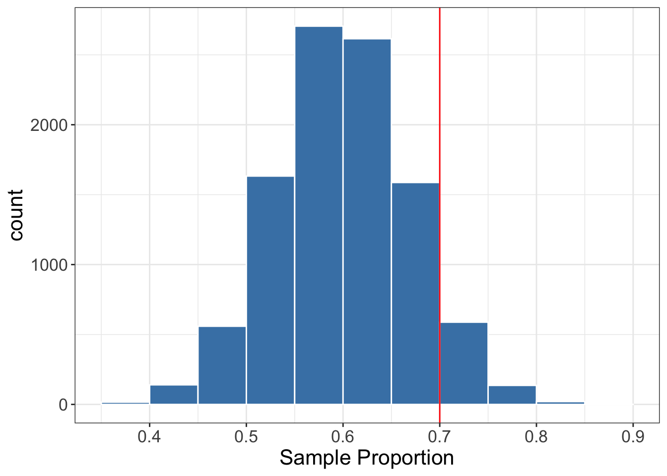
Suppose we take a sample of 50 patients and observe whether they are protected from the flu by the new vaccine. Since we are testing the population proportion, let us use the sample proportion as the test statistic for this test. Now, if H_0 is true what is the sampling distribution of \hat{p}? This is the null model and it is shown in Figure 6.6.
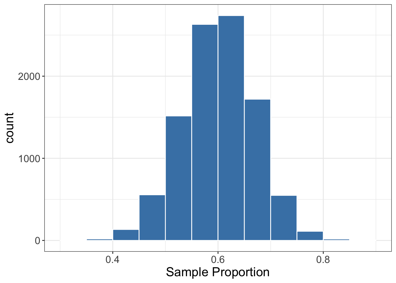
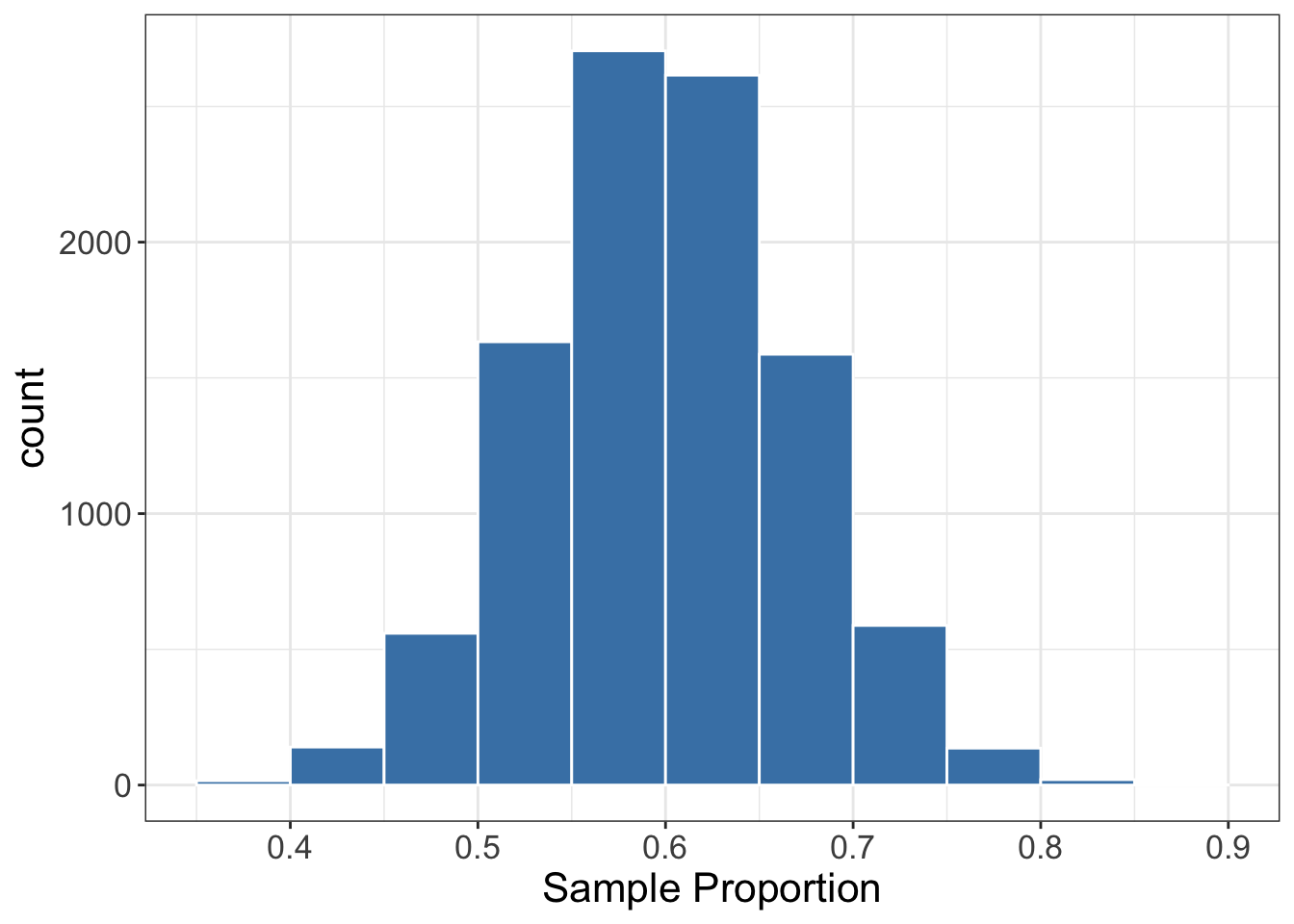
Great! According to the null model (i.e., assuming H_0 is true), we would expect to observe a \hat{p} around 0.5 and 0.7. If we end up observing a \hat{p}, say, around 0.9, we are either very “unlucky” or H_0 is not true. Imagine we obtained a sample proportion \hat{p}=35/50=0.7 as shown in Figure 6.7.
To calculate the p-value we want the probability of observing a \hat{p} being at least as extreme as the one we observed (i.e., 0.7). under the null model in favour of the alternative hypothesis. We know that the alternative hypothesis states that p>0.6. So the “alternative” side of the distribution is the right side. The p-value is the area to the right of the observed test statistic. This is shown in Figure 6.8.
In this case, the p-value is 0.0685. This means that if H_0 is true, only 6.85\% of the possible samples would yield a \hat{p} of 0.7 or higher. Is this too rare, suggesting that H_0 is false? To answer this question, we need to compare the p-value to the significance level. If the p-value is less than the significance level, we reject H_0. Otherwise, we do not have enough evidence to reject H_0.
□
Important
p-value is a conditional probability. Conditioned on H_0 being true. This condition comes into play because we use the null model to calculate the p-value.
Next, let’s break down the definition of p-value:
The p-value is the \underbrace{\text{probability, under the null model}}_{\#1}, of observing a \underbrace{\text{test statistic at least as extreme as the one observed in the sample data}}_{\#2}, \underbrace{\text{in favour of }H_A}_{\#3}.
Let’s dissect this definition:
\#1: The p-value is a probability, which means it ranges from 0 to 1. We can calculate as the area under the curve in mathematical models, or counting the proportions of points in simulation-based methods.
\#2: This tells us the threshold for “extreme”, which is the observed test statistic.
\#3: This part brings the alternative hypothesis into play. It defines the direction that we consider “extreme”. The area on the right? on the left? or both sides?
The point \#3 above determines the type of test we are conducting. There are three types of tests:
Left-tailed test (H_A: \theta < \theta_0)
If the alternative hypothesis is of the form H_A: \theta < \theta_0, where \theta is any parameter of interest, the p-value is the area on the left of the observed test statistic (including the test statistic), as shown in Figure 6.9 below.
Right-tailed test (H_A: \theta > \theta_0)
If the alternative hypothesis is of the form H_A: \theta > \theta_0, where \theta is any parameter of interest, the p-value is the area on the left of the observed test statistic (including the test statistic), as shown in Figure 6.10.
Two-tailed test (H_A: \theta \neq \theta_0)
Now consider the alternative hypothesis is of the form H_A: \theta \neq \theta_0, where \theta is any parameter of interest. To calculate the p-value in this case, we follow these four steps:
- Calculate the p-value as if the test were a right-tailed test: \text{p-value}_{\text{right}}.
- Calculate the p-value as if the test were a left-tailed test: \text{p-value}_{\text{left}}.
- Select the smaller of \text{p-value}_{\text{right}} and \text{p-value}_{\text{left}}, then multiply it by 2.
- Finally, since the p-value is a probability, ensure it does not exceed 1.
In mathematical terms, this can be expressed as: \text{p-value} = \min\{1, 2\text{p-value}_{\text{right}}, 2\text{p-value}_{\text{left}}\}. This approach is called twice-the-smaller-tail (Thulin 2024).
6.3.6 Exercises
Exercise 6.3
A coffee shop claims their average wait time is 3 minutes. A customer advocacy group believes the wait time is longer. H_0: \mu = 3 \quad\quad \text{vs}\quad\quad H_A:\mu > 3 The test statistic: \bar{X}\sim N(3, 0.5^2). In a sample of 100 costumers, the observed sample mean was \bar{x} = . Calculate the p-value.
#| exercise: exr_6_3_1
#| input:
#|   - exr_6_3_1_xbar
p_value = ...
#| exercise: exr_6_3_1
#| check: true
#| input:
#| - exr_6_3_1_xbar
if (identical(.result, 1-pnorm(exr_6_3_1_xbar, 3, 0.5))) {
list(correct = TRUE, message = "Nice work!")
} else {
list(correct = FALSE, message = "That's incorrect, sorry. Try checking the hint!")
}
Hint 1
You want the following area under the curve.
#| edit: false
#| echo: false
#| input:
#|   - exr_6_3_1_xbar

# Create a data frame with x values
data <- tibble(x = seq(1, 5, 0.01),
               y = dnorm(x, 3, 0.5))

# Create the plot
ggplot(data, aes(x = x, y = y)) +
  geom_line() +
  geom_area(data = subset(data, x >= exr_6_3_1_xbar), fill = "red") +
  labs(title = "Null model (Normal Distribution)",
       x = "Sample Mean",
       y = "Density") +
  theme_minimal()
Which function should you use to get the area under the Normal curve: qnorm or pnorm?
Exercise 6.4 More coming soon!!
6.4 Simulation-based hypothesis testing
The challenging aspect of hypothesis testing lies in identifying the test statistic and its null model. The null model represents the sampling distribution of the test statistic, assuming the null hypothesis is true. As we have seen before, we can investigate the sampling distribution of the test statistic via simulation-based approaches and mathematical approximations.
In this chapter, we will concentrate on simulation-based methods, while the mathematical approach will be covered in the next chapter. The fundamental idea behind simulation-based methods is to simulate values from the null model and use these simulated values to approximate the p-value.
6.4.1 One population
In this section, we will focus on problems involving a single parameter of a given population.
Test for one mean (\mu)
Let us go back again to Example 6.1. During the summer, Vancouver’s beaches get pretty busy. To ensure everybody’s safety, the city of Vancouver monitors if the beaches’ waters are safe for swimming. To test the water quality of a beach, the city of Vancouver takes multiple samples of the water and calculates the average number of E. coli (bacteria) per 100 mL. If the average number of E. coli per 100mL is 400 or less, the city considers the beach proper for swimming. Otherwise, the city of Vancouver releases a warning to let people know that they should not swim on the beach. The city wants to test if the water is unsafe.
Suppose that right before the summer, the city of Vancouver is going to test the water at Kitsilano Beach. Given the cost of closing a beach, the City of Vancouver wants to do that only if there’s strong evidence that they should do it.
Steps 1 & 2: Set the hypotheses and significance level
They set the hypotheses: H_0: \mu = 400\quad\quad\text{vs}\quad\quad H_A: \mu > 400 and want to test at a 10\% significance level.
To test the hypothesis, the technicians took 59 samples of 100 mL at different points of the beach. The data is available in the variable kits_sample in the code cell below.
#| output: false
#| autorun: true
#| edit: false
#|
set.seed(1)

kits_ecoli_sample <- rnorm(59, 415, 85.68)
kits_sample <- tibble(
  e_coli = round(kits_ecoli_sample - mean(kits_ecoli_sample) + 415)
)

sample_mean <- mean(kits_sample$e_coli)
sample_sd <- sd(kits_sample$e_coli)
####################################
# Sample data from Kitsilano Beach #
####################################
kits_sampleLet’s examine the sample data more closely.
##############################################
# Calculate sample mean and sample std. dev. #
##############################################
sample_mean <- mean(kits_sample$e_coli)
sample_sd <- sd(kits_sample$e_coli)

# Print the value of the statistics
cat("Sample mean:", sample_mean)
cat("Sample std. dev.:", sample_sd)

################################
# Plot the sample distribution #
################################
kits_sample %>%
  ggplot() +
  geom_histogram(aes(e_coli),
                 color = 'white',
                 fill = 'steelblue',
                 bins = 10) +
  ggtitle("Sample Distribution of E. Coli per 100mL in 59 samples from Kitsilano Beach") +
  xlab('E. Coli') +
  theme_bw()
Step 3: Defining the test statistic
Now that we have the data, we need to determine if our sample is “compatible” with the null hypothesis. The null hypothesis states that the population mean is equal to 400 E. coli. Therefore, if the null hypothesis is true, we would expect the sample mean to be close to 400. This suggests that the sample mean is a reasonable test statistic in this context. But how close does the sample mean need to be to 400? To answer this question, we must consider what the sampling distribution of the sample would look like if the null hypothesis were true; this represents the null model.
Step 4: Obtaining the null model
We learned that we can use bootstrapping to approximate the sampling distribution of \bar{X}.
set.seed(1)
#######################################
# Generate the bootstrap distribution #
# based on kits_sample.               #
#######################################
boot_dist <-
  kits_sample %>%
  rep_sample_n(size = 59, replace=TRUE, reps = 10000) %>%
  summarise(xbar = mean(e_coli))

###################################
# Plot the bootstrap distribution #
###################################
boot_dist %>%
  ggplot() +
  geom_histogram(aes(xbar),
                 color = 'white',
                 fill = 'steelblue',
                 bins = 20) +
  ggtitle('Bootstrap Distribution') +
  xlab('Avg. E. Coli per 100mL') +
  theme_bw()
The issue with the Bootstrap Distribution generated above is that it attempts to approximate the true sampling distribution, rather than representing the sampling distribution when the null hypothesis H_0 is true, which corresponds to the null model. Therefore, if H_0 is false, the Bootstrap distribution does not reflect the null model.
To adapt our code to generate samples from the null model instead of the sampling distribution, we need to incorporate the information provided by the null hypothesis. In this example, the null hypothesis asserts that \mu = 400, indicating that the mean of the null model is 400. To create our null model, we can shift our sample distribution so that its mean is 400. Remember, the mean of the boostrap distribution in this case is the sample mean, so this shift will make the bootstrap distribution to be centered at 400 as specified by our null hypothesis. The code is very similar to generate the bootstrap distribution with only one extra step that centers the sample distribution at \mu_0 (in this case \mu_0 = 400).
set.seed(1)
##################################################
# Approximating the null model via Bootstrapping #
##################################################
null_model <-
  kits_sample %>%
  mutate(e_coli = e_coli - mean(e_coli) + 400) %>%
  rep_sample_n(size = 59, replace=TRUE, reps = 10000) %>%
  summarise(xbar = mean(e_coli))

#######################
# Plot the null model #
#######################
null_model %>%
  ggplot() +
  geom_histogram(aes(xbar),
                 color = 'white',
                 fill = 'steelblue',
                 bins = 20) +
  ggtitle('Null model via Simulation') +
  xlab('Avg. E. Coli per 100mL') +
  theme_bw()
As you can see, the only difference here is the inclusion for the line mutate(e_coli = e_coli - mean(e_coli) + 400). Here’s how it works:
The expression e_coli - mean(e_coli) centers the mean of the sample at 0. The spread remains the same. By adding 400 to this result, we shift the mean of the sample to 400. In other words, e_coli - mean(e_coli) + 400 makes the sample mean to be 400. Again, the mean of the boostrap distribution in this case is the sample mean, which now will be 400, as specified in H_0. Therefore, the distribution above is the sampling distribution of \bar{X} when the null hypothesis is true, i.e., the null model. We are just shifting the bootstrap distribution as shown in the plot below.
###################################################
# We have just shifted the bootstrap distribution #
# to be centred at μ0.                            #
###################################################
ggplot() +
  geom_histogram(data = boot_dist, aes(x=xbar, fill = "Bootstrap Dist."),
                 bins = 20, color = "black") +
  geom_histogram(data = null_model, aes(x=xbar, fill = "Null Model"),
                 bins = 20, color = 'white', alpha = 0.5) +
  scale_fill_manual(values = c('Bootstrap Dist.'='steelblue', 'Null Model'='red'))+
  theme_bw()
Step 5: Calculate the p-value
At this point, we understand how our test statistic, \bar{X}, behaves if H_0 is true. But how does the observed value of the test statistic in our specific sample compare to the null model? Specifically, we want to determine how likely it is to obtain a value for the test statistic that is equal to or greater than our observed mean.
##################################################
# Plot the null model vs Observed Test Statistic #
##################################################
null_model %>%
  ggplot() +
  geom_histogram(aes(xbar),
                 color = 'white',
                 fill = 'steelblue',
                 bins = 20) +
  geom_vline(aes(xintercept = sample_mean), color='red') +
  annotate("rect",
           xmin = sample_mean, xmax = Inf,
           ymin = -Inf, ymax = Inf,
           alpha = .2,
           fill = 'red') +
  ggtitle('Null model via Simulation vs Test Statistic') +
  xlab('Avg. E. Coli per 100mL') +
  theme_bw()
The observed test statistic is positioned at the right tail of the null model, indicating that such a high sample average is somewhat unlikely to occur when the null hypothesis is true. But just how unlikely is it? To determine this, we can calculate the proportion of all possible samples that would result in a sample average at least as high as the one we observed if the null hypothesis were true. This value is known as the p-value.
#####################
# Calculate p-value #
#####################
(pvalue <- mean(null_model$xbar >= sample_mean))

# Note that here, we are checking whether the
# mean generated from the null model is
# higher than or equal to the mean in our sample.
This means that if H_0 were true, only 5% of the samples would give us a sample mean as high as or higher than the observed sample mean. Were we very unlucky of selecting such a rare sample, or is H_0 false? To make this decision we compare the p-value against the significance level. For example, for a significance level of \alpha = 10\%, we have that \text{p-value} < \alpha, and we reject H_0. In this case we say:
There is enough evidence at 10\% significance level to reject the hypothesis that the average count of E. Coli per 100 mL in the Kitsilano beach is 400 in favour of the alternative hypothesis that the average is higher than 400.
If instead we were to use \alpha = 5\%, we have that \text{p-value} > \alpha, and in this case, we would not reject H_0:
There is not enough evidence at 5\% significance level to reject the null hypothesis that the average count of E. Coli per 100 mL in the Kitsilano beach is 400 in favour of the alternative hypothesis that the average is higher than 400.
It is important to note that the significance level must be defined before looking at the data. You must not adjust your significance level to reach the conclusion you desire.
The infer workflow
Although the workflow above is helpful for us to explore the process of simulation-based hypothesis testing, the infer package (Couch et al. 2021) provides a more convenient way to do this, which is very similar to the workflow we have used for confidence intervals. To simulate from the null model, we just need to add one extra line.
set.seed(1)
###########################################
# Infer workflow: generate the null model #
###########################################
null_model_infer <-
  kits_sample %>%
  specify(response = e_coli) %>%
  hypothesize(mu = 400, null = 'point') %>%
  generate(reps = 20000, type = 'bootstrap') %>%
  calculate(stat = 'mean')

# Let's take a look:
null_model_infer %>% head()
The only function from this workflow we haven’t seen before is the hypothesize function. The hypothesize function defines the null hypothesis (i.e., we define the parameter of interest and its value under H_0). In this case, we are saying: null = point, which tells infer that we want to test only one parameter (the point it is because we are testing if the parameter is equal to one value – a point in the real line). To specify the parameter to be tested and its value under H_0, we passed mu = 400. The mu says that we are testing the mean (we could have said p = ... [for proportion] or med = ... [for the median]), and 400 specifies the value of \mu_0.
The variable null_model_infer stores the simulated values from the null model. To get the p-value, we can use the get_p_value function (or its alias get_pvalue). For the get_p_value function, you need to specify the observed test statistic and the direction of the test, in this case the observed sample mean and right-tailed test.
###############################
# Infer workflow: get p-value #
###############################
null_model_infer %>%
  get_p_value(sample_mean, direction = 'right')
Finally, to visualize the test, we can use the visualize function combined with the shade_pvalue.
##################################################
# Infer workflow: visualize the test and p-value #
##################################################
null_model_infer %>%
  visualize() +
  shade_pvalue(sample_mean, direction = 'right')
Test for one median (Q_{0.5})
The case of the median is very similar to the mean. Let’s go over the procedures with an example.
Example 6.11 A Senate hearing is currently investigating consumer complaints regarding airlines in the United States. During one of the sessions, the CEO of American Airlines was questioned about the time it takes for the company to resolve customer support tickets. The CEO stated that the median resolution time is 48 hours, indicating that 50% of the tickets are resolved in 48 hours or less. In response to this claim, the Senate hearing committee decided to conduct a further investigation. They collected a sample of 100 support tickets and examined the resolution times in hours, which are recorded in the support_time variable.
#| autorun: true
#| output: false
#| edit: false
set.seed(1)

support_time <- tibble(
  time_hrs = 18 * (abs(rt(100, 1))+2)
)

supp_time_median <- median(support_time$time_hrs)
####################################
# Sample data from support tickets #
####################################
support_time %>% head()
############################
# Plot sample distribution #
############################
support_time %>%
ggplot() +
geom_histogram(aes(time_hrs),
color = 'white',
fill = 'steelblue',
bins = 20) +
xlab("Resolution Time (hrs)") +
ggtitle("Sample distribution of American Airline support tickets") +
theme_bw()Steps 1 & 2: Set the hypotheses and significance level
The senate will test the hypothesis H_0: Q_{0.5} = 48 \quad\quad vs \quad\quad H_A: Q_{0.5} > 48 and if there is enough evidence at 5\% significance level, the senate will issue a fine to American Airlines.
Step 3: Defining the test statistic
Since we are testing the population median, it’s sensible to use the sample median as our test statistic.
#######################################
# Compute the observed test statistic #
#######################################
(supp_time_median <- median(support_time$time_hrs))
Step 4: Obtaining the null model
Next, we will simulate values from the null model. We cannot simply resample from our sample because this approach will not accurately represent the null model if the null hypothesis (H_0) is false. However, similar to how we might adjust for the mean, we can shift our sample so that the median matches the value specified in H_0, which is 48 hours.
set.seed(2)
##################################################
# Approximating the null model via Bootstrapping #
##################################################
null_model_supp_time <-
  support_time %>%
  mutate(time_hrs = time_hrs - median(time_hrs) + 48) %>%
  rep_sample_n(size = 100, reps = 15000, replace = TRUE) %>%
  summarise(q_50 = median(time_hrs))
Step 5: Calculate the p-value
Finally we can calculate the p-value.
set.seed(2)
##########################
# Calculate the p-value. #
##########################
(p_value <- mean(null_model_supp_time$q_50 > supp_time_median))
Since the p-value is approximately 31%, the Senate does not have enough evidence at a 5% significance level to reject the American Airlines CEO’s claim that the median time to resolve a support ticket is 48 hours.
The infer workflow
Again, the infer workflow makes this entire analysis more convenient. To generate from the null model using the infer workflow:
###########################################
# Infer workflow: generate the null model #
###########################################
null_model_supp_time_infer <-
  support_time %>%
  specify(response = time_hrs) %>%
  hypothesise(null = 'point', med = 48) %>%
  generate(reps = 15000, type = "bootstrap") %>%
  calculate(stat = "median")
Next, we obtain the p-value.
##################################
# Infer workflow: Obtain p-value #
##################################
null_model_supp_time_infer %>%
  get_p_value(obs_stat = supp_time_median, direction = 'right')
Finally, the visualize function gives us an overall picture of the test.
##################################
# Infer workflow: visualize test #
##################################
null_model_supp_time_infer %>%
  visualise() +
  shade_pvalue(obs_stat = supp_time_median, direction = 'right')
□
Test for one proportion (p)
Suppose we want to test H_0: p = p_0 against one of H_A: p\neq p_0, H_A: p > p_0, or H_A: p < p_0. Since we want to test the proportion, it is natural to use the sample proportion as our test statistic.
Here, again, we want to simulate the null distribution. However, the procedure differs slightly from the mean and median one. This is because, for proportion, we cannot simply shift the distribution. Remember that the standard error of \hat{p} is given by SE(\hat{p}) = \sqrt{\frac{p(1-p)}{n}}, which depends on p. So, it is not possible for us to shift the sample distribution without also affecting the standard error of the statistic.
However, in the case of proportions, we know that every element in our population is either a 0 (indicating that they do not possess the attribute we are examining) or a 1 (indicating that they do possess the attribute) as illustrated in Figure 6.11.

The challenge is that, since we don’t have access to the population, we do not know the exact proportion of each category. Essentially, it is like having a bar chart with one bar representing zeros and another for ones, but we simply do not know the height of each bar.
Luckily for us, H_0: p = p_0 tell us exactly the size of each of the bar if the null hypothesis were true. So, we know exactly what our population would look like under H_0. Therefore, we can draw new values directly from the population under the null hypothesis, and we don’t need to resample from our sample.
Example 6.12 According to the National Institute of Diabetes and Digestive and Kidney Diseases, approximately 42.5% of adults in the United States are classified as obese. The new Health Secretary aims to launch a campaign that encourages Americans to adopt better eating habits and lead healthier lifestyles. As part of this initiative, a series of new policies has been implemented. After two years, the House of Representatives plans to evaluate the effectiveness of the program to determine if there has been any change in the obesity rate. They have surveyed a random sample of 300 adults, with the data available in the obesity_study variable. The objective is to test the hypothesis: H_0: p = 0.425 versus H_A: p \neq 0.425 at a 5\% significance level.
#| edit: false
#| output: false
#| echo: false
#| autorun: true

set.seed(1)
obesity_study <- tibble(
  is_obese = rbinom(300, size = 1, prob = 0.40)
) %>%
  mutate(is_obese = if_else(is_obese == 1, "yes", "no"))
sample_prop_obese <- mean(obesity_study$is_obese == "yes")
#############################
# Sample data obesity study #
#############################
obesity_study
(sample_prop_obese <- mean(obesity_study$is_obese == "yes"))To test the hypotheses, we will use the sample proportion. Our next step is to generate value from the null model. But note that H_0 specifies what our population looks like. So, to “estimate” the null model, we can take multiple samples directly from this would-be population if H_0 were true. To sample from this distribution, we randomly select between "yes" or "no" with the probability of "yes" equals to p_0=0.425.
#####################################
# Storing the values of the problem #
#####################################
sample_size = 300
reps = 10000
p0 = 0.425

################################################
# Null model: two steps                        #
#   1. Take multiple samples from the          #
#      theoretical population (under H0);      #
#   2. Calculate the sample proportion of each #
#      sample to obtain the null model.        #
################################################
null_model_obesity <- tibble(
    replicate = rep(1:reps, sample_size),
    is_obese = sample(c('yes', 'no'),
                      size = sample_size * reps,
                      prob = c(p0, 1-p0),
                      replace = TRUE)
  ) %>%
  group_by(replicate) %>%
  summarise(sim_phat = mean(is_obese == 'yes'))

null_model_obesity
Let’s examine the null model and the observed test statistics.
#####################################
# Plot the simulated null model and #
# the observed test statistic.      #
#####################################
null_model_obesity %>%
  ggplot() +
  geom_histogram(aes(x = sim_phat),
                 fill = 'steelblue',
                 color = 'white',
                 bins = 15) +
  geom_vline(xintercept = sample_prop_obese, color = 'red') +
  ggtitle('Null Model via Simulation') +
  xlab('Simulated proportions') +
  theme_bw()
In the plot above, we can see that the test statistic is located on the left side. This means that our sample proportion of obese individuals, as \hat{p} = 0.37, is smaller than the hypothesized proportion p_0 = 0.425. To calculate the p-value, we determine the proportion of simulated statistics that fall below our \hat{p} = 0.37 and then multiply that proportion by 2.
###############
# Get p-value #
###############
null_model_obesity %>%
  summarise(p_value = 2 * mean(sim_phat <= sample_prop_obese))
Therefore, at a 5\% significance level, we fail to reject H_0. The conclusion is :
The House of Representatives doesn’t have enough evidence to reject the null hypothesis that the obesity proportion is 42.5\% in favour of H_A, that the obesity proportion is different from 42.5\%.
Finally, once again, the infer workflow makes our life much easier. Let us take a look.
###########################################
# Infer workflow: generate the null model #
###########################################
null_model_obesity_infer <-
  obesity_study %>%
  mutate(is_obese = is_obese) %>%
  specify(response = is_obese, success = 'yes') %>%
  hypothesise(null = 'point', p = 0.425) %>%
  generate(reps = 10000, type = 'draw') %>%
  calculate(stat = 'prop')
There are two differences from the previous approach we used for the mean:
- First, note that when we call
specify, we must now define what is considered “success”. For this study we havespecify(response = is_obese, success = "yes"). - Second, we need to specify that we want to generate from a theoretical population instead of resampling from the original sample. Therefore, in the
generatefunction, we usetype = "draw".
The code above generates values from the theoretical population distribution if H_0 were true. Next, we can calculate the p-value and visualize the test.
##################################
# Infer workflow: visualize test #
##################################
null_model_obesity_infer %>%
  visualize() +
  shade_pvalue(obs_stat = sample_prop_obese, direction = 'both')

###############################
# Infer workflow: get p-value #
###############################
(p_value_obese_infer <- null_model_obesity_infer %>%
  get_p_value(obs_stat=sample_prop_obese, direction = 'both'))
□
6.4.2 Two populations
In this section, we will discuss comparing two parameters. We will focus on the difference of means or proportions. Let’s see a couple of examples.
Example 6.13 A common claim is that Alberta is more conservative than British Columbia (BC). Is this true regarding federal politics? Ahead of the next Federal Election, Nanos Research is polling Canadian voters. In a random sample of 200 British Columbians, 80 said they would vote for the Conservative Party of Canada. In contrast, in a random sample of 300 Albertans, 150 said they would vote for the Conservative Party. We want to test H_0: p_{\text{Alberta}} - p_{\text{BC}} = 0 vs H_A: p_{\text{Alberta}} - p_{\text{BC}} > 0.
□
Example 6.14 The Flying Falcons, based in Boulder, Colorado, have a training program that heavily emphasizes plyometrics and high-altitude training. Their philosophy centers around maximizing explosive power through intense, short-duration workouts. The Cheetah Striders, located in Eugene, Oregon, take a different approach. Their training regimen focuses on a combination of strength training (with a focus on Olympic lifting) and sprint mechanics, with longer, more varied workout sessions designed to build both power and endurance.
We want to investigate whether there’s a statistically significant difference in the average vertical jump height between athletes from these two clubs. We will test H_0: \mu_{\text{Falcons}} - \mu_{\text{Striders}} = 0 vs H_0: \mu_{\text{Falcons}} - \mu_{\text{Striders}} \neq 0. This study might influence training strategies and talent scouting.
□
To test the hypothesis of differences in means or proportions, we will generate values from the null model using a permutation strategy. This approach involves randomly rearranging the two groups to create balance.
To illustrate the concept of the permutation strategy, imagine you have two pots of soup: one is very salty, while the other lacks salt. You combine both pots into a larger pot, mix them thoroughly, and then refill the original two pots from the mixed pot. After doing this, you would expect both pots to have a similar amount of salt, right? That’s the idea of permutation.
Example 6.15 Suppose we want to study if the proportion of students who drink coffee is the same among graduate and undergraduate students. To examine this, we randomly select a sample of four graduate students and four undergraduate students.

The idea of permutation is to randomly shuffle the students across the groups. This means that some undergraduate students may join the graduate students’ group and vice versa. Essentially, we treat all students as one large group and then randomly assign them to smaller groups.

Next, since we are randomly splitting all of the students (combined) into two separate groups, there’s no reason for us to expect one group to have a consistently higher proportion of students who drink coffee than the other group. Of course, if you do this one time, it could happen, just by chance, that one group has a higher proportion than the other. But if you made many of such splits, neither group would consistently have a higher proportion of students who drink coffee.
So, the permutation strategy allows us to use our samples to generate values from the null model (that both groups are equal), even when our sample data has unequal groups (like in this case). Cool, isn’t it?
□
As you can see in Example 6.15, by repeating the permutation process numerous times, we generate a large set of potential outcomes that reflect what we would expect if the null hypothesis were true. We can then compare our observed test statistic (the difference in means or proportions) against this distribution to determine how extreme our observed statistic is.
Difference in proportions (p_1-p_2)
Suppose we want to assess the success rates of two different surgical procedures used to treat severe carpal tunnel syndrome: “Endoscopic Carpal Tunnel Release” (ECTR) and “Mini-Open Carpal Tunnel Release” (MOCTR). Both procedures aim to relieve pressure on the median nerve in the wrist, but they differ in their approach.
Step 1: Formulate the hypotheses
In this case, we want to check whether both surgeries have the same probability of success. In other words, H_0: p: p_{\text{MOCTR}} - p_{\text{ECTR}} = 0\quad\quad vs\quad\quad H_A: p: p_{\text{MOCTR}} - p_{\text{ECTR}} \neq 0
Step 2: Define the significance level
Let’s use a significance level of \alpha = 10\%.
We collected data from 10 patients for the ECTR surgery and 8 patients for the MOCTR surgery. For ECTR, eight patients (out of 10) successfully recovered. However, for the MOCTR, only two patients (out of 8) successfully recovered.
Let’s continue with our surgery example from the previous section. The data is available in the surgery_data object below.
#| echo: false
#| edit: false
#| output: false
set.seed(1)
surgery_data <- tibble(surgery = c(rep('MOCTR', 8), rep('ECTR', 10)),
             recovered = as_factor(c(rep("yes", 2), rep("no", 8), rep("yes", 8)))) %>%
      slice_sample(prop = 1)
################
# Surgery Data #
################
surgery_data
################################
# Plot the sample distribution #
################################
surgery_data %>%
ggplot(aes(x = recovered, fill = surgery)) +
geom_bar(position='dodge') +
ggtitle("Recover counts per surgery type") +
theme_bw() +
theme(text = element_text(size=14))Step 3: Define the test statistic
Since we are testing the difference in probabilities, let’s use the difference in sample proportions as our test statistic: Z = \hat{p}_{\text{MOCTR}} - \hat{p}_{\text{ECTR}}
#######################################
# Compute the observed test statistic #
#######################################
obs_test_statistic_surgery <-
  surgery_data %>%
  specify(recovered ~ surgery, success = 'yes') %>%
  calculate(stat = "diff in props", order = c("MOCTR", "ECTR"))

obs_test_statistic_surgery
Step 4: Obtain the null model
In this step we need to generate values from the null model so we can understand how our test statistic would behave if the null hypothesis were true. To do this, we will use the infer package.
###########################################
# Infer workflow: generate the null model #
###########################################
null_model_surgery <-
  surgery_data %>%
  specify(recovered ~ surgery, success = 'yes') %>%
  hypothesise(null = 'independence') %>%
  generate(reps = 10000, type = 'permute') %>%
  calculate(stat = "diff in props", order = c("MOCTR", "ECTR"))

null_model_surgery
We have a very similar workflow but some new arguments. Let’s discuss them line-by-line.
Line 6 –
specify(recovered ~ surgery, success = 'yes'): in this command, we are using the formularecovered ~ surgery. This formula tellsinferthat we want to explain the response variablerecoveredusing the explanatory variablesurgery. In this case, we are separatingrecoveredinto two groups (one for each surgery).Line 7 –
hypothesize(null = 'independence'): this command specifies the null hypothesis, saying that we want to check ifrecoveredis independent ofsurgery. In other words, thesurgerymethod doesn’t affect the probability ofyesinrecovered.Line 8 –
generate(reps = 10000, type = 'permute'): here we usetype = 'permute'to follow the permutation approach discussed in the previous section.Line 9 –
calculate(stat = "diff in props", order = c("MOCTR", "ECTR")): the order argument defines whether we want to calculate \hat{p}_{\text{MOCTR}} - \hat{p}_{\text{ECTR}} or \hat{p}_{\text{ECTR}}-\hat{p}_{\text{MOCTR}}. In this case, we used the former.
Step 5: calculate p-value
###############################
# Infer workflow: get p-value #
###############################
null_model_surgery %>%
  get_p_value(obs_stat = obs_test_statistic_surgery, direction = 'both')
Since the p-value is lower than \alpha = 10\%, we reject the null hypothesis at a 10% significance level.
We have enough evidence at a 10% significance level to reject the null hypothesis that both surgery approaches, MOCTR and ECTR, have the same probability of successful recovery.
□
Difference in means (\mu_1-\mu_2)
The workflow to test the differences in means (or in medians for that matter) is exactly the same as for the differences in proportion. To illustrate hypothesis testing for the difference in means, let’s go back to Example 6.6.
Step 1: Formulate the hypotheses
In this case, we want to check whether both fertilizers yields the same growth. In other words, H_0: \mu_{\text{GF}}-\mu_{\text{BB}}=0 \quad\quad \text{ vs } \quad\quad H_A: \mu_{\text{GF}}-\mu_{\text{BB}}\neq0 where \mu_{\text{GF}} is the mean height of plants using Fertilizer GrowFast, and \mu_{\text{BB}} is the mean height of plants using Fertilizer BloomBoost.
Step 2: Define the significance level
Let’s use a significance level of \alpha = 10\%.
A batch of 30 tomato plants received the Fertilizer GrowFast, and another batch of 30 tomato plants received the Fertilizer BloomBoost. The data is available in the fertilizer_data variable.
#| echo: false
#| edit: false
#| output: false
set.seed(1)
fertilizer_data <-
  tibble(
    fertilizer = c(rep('GrowFast', 30), rep('BloomBoost', 30)),
    height = rnorm(60, 90, 3)) %>%
  mutate(height = if_else(fertilizer == 'BloomBoost', height + 3, height)) %>%
  slice_sample(prop = 1)
###################
# Fertilizer Data #
###################
fertilizer_data
################################
# Plot the sample distribution #
################################
fertilizer_data %>%
ggplot(aes(x = fertilizer, y = height, fill = fertilizer)) +
geom_boxplot() +
ggtitle("Growth of tomato plants per fertilizer") +
theme_bw() +
theme(text = element_text(size=14))Step 3: Define the test statistic
Since we are testing the difference in means, let’s use the difference in sample means as our test statistic: T = \bar{X}_{\text{GF}} - \bar{X}_{\text{BB}}
#######################################
# Compute the observed test statistic #
#######################################
obs_test_statistic_fertilizer <-
  fertilizer_data %>%
  specify(height ~ fertilizer) %>%
  calculate(stat = "diff in means", order = c("GrowFast", "BloomBoost"))

obs_test_statistic_fertilizer
Step 4: Obtain the null model
In this step we need to generate values from the null model so we can understand how our test statistic would behave if the null hypothesis were true. To do this, we will use the infer package.
###########################################
# Infer workflow: generate the null model #
###########################################
null_model_fertilizer <-
  fertilizer_data %>%
  specify(height ~ fertilizer) %>%
  hypothesise(null = 'independence') %>%
  generate(reps = 10000, type = 'permute') %>%
  calculate(stat = "diff in means", order = c("GrowFast", "BloomBoost"))

null_model_fertilizer
Step 5: calculate p-value
###############################
# Infer workflow: get p-value #
###############################
null_model_fertilizer %>%
  get_p_value(obs_stat = obs_test_statistic_fertilizer, direction = 'both')
Since the p-value is lower than \alpha = 1\%, we reject the null hypothesis at a 1\% significance level.
We have enough evidence at a 1% significance level to reject the null hypothesis that both fertilizers, GrowFast and BloomBoost, yield the same growth of tomato plants.
Caution
Note that, in this case, the get_p_value function returned a p-value of 0 along with a warning message. This warning is important because a p-value should not be exactly 0. The root of the issue lies in how we are approximating the null model through simulation, which involves generating a large number of test statistics under the null hypothesis—in this case, 10,000. We then count how many of these generated statistics are “more extreme” than the observed test statistic, but in this instance, none were. As a result, our approximation of the p-value turned out to be 0.
However, the true p-value is actually very small (around 0.000015). To achieve a better approximation, it would be necessary to generate a much larger sample size, such as 1,000,000 values (unfortunately, this will not work quite well in this browser environment) Therefore, it’s essential to exercise caution. The fact that we estimated the p-value to be zero may simply indicate that the true p-value is smaller than 1/\text{reps}—in this case, 1/10,000—rather than being precisely 0.
6.4.3 Exercises
Coming soon!
6.5 Take-home points
Coming soon!