library(dplyr)
library(tidyverse)
library(infer)
library(gsDesign)12 STAT 201 Concept Cheatsheet
13 Set-up
Load important packages to be able to run examples.
Throughout this cheatsheet we will use the Palmer penguin dataset to show examples of code. This dataset is found in the R package palmerpenguins.
library(palmerpenguins)We will focus mostly on the flipper length (mm) of two penguins species: Chinstrap and Adelie. Thus, we will create new tbl called adelie and chinstrap.
adelie <- penguins %>%
  filter(!is.na(flipper_length_mm) &
           species == "Adelie" & !is.na(sex)) %>%
  droplevels() %>%
  dplyr::select(species, flipper_length_mm, sex)

chinstrap <- penguins %>%
  filter(!is.na(flipper_length_mm) &
           species == "Chinstrap" &
           !is.na(sex)) %>%
  droplevels() %>%
  dplyr::select(species, flipper_length_mm, sex)
Using the penguins_raw dataset, we will also look at changes in body mass for Gentoo penguins that were captured on Biscoe Island in 2008 and recaptured on the same Island in 2009.
gentoo_mass_diff <- penguins_raw %>%
  filter(Species == "Gentoo penguin (Pygoscelis papua)" &
           Island == "Biscoe" & !is.na("Body Mass (g)")) %>%
  droplevels() %>%
  rename( "ID" = `Individual ID`, "Body_mass_g" = `Body Mass (g)`) %>%
  mutate(Year =
           as.numeric(paste("20", substring(studyName, 4, 5), sep = ""))) %>%
  filter(Year == 2008 | Year == 2009) %>%
  filter(duplicated(ID, fromLast = TRUE) | duplicated(ID) ) %>%
  select(ID, Body_mass_g, Sex, Year) %>%
  arrange(ID)
14 Section 1: Standard Error
| Sample statistic | Theory | Estimate | Method |
|---|---|---|---|
| General (\hat{\theta}) | \sigma_{\hat{\theta}} = \sqrt{\sum_{j=1}^K (\hat{\theta}_j - \theta)^2/K} | \hat{\sigma}_{\hat{\theta}} = \sqrt{\sum_{j=1}^K (\hat{\theta}_j^* - \hat{\theta})^2/(K - 1)} | Bootstrap |
| Sample mean (\bar{X}) | \sigma_{\bar{X}} = \frac{\sigma}{\sqrt{n}} | \hat{\sigma}_{\bar{X}} = \frac{s}{\sqrt{n}} | Traditional/math |
| Sample proportion (\hat{p}) | \sigma_{\hat{p}} = \sqrt{\frac{p \times (1-p)}{n}} | \hat{\sigma}_{\hat{p}} = \sqrt{\frac{\hat{p} \times (1-\hat{p})}{n}} | Traditional/math |
Notation:
- \theta: population parameter
- \sigma: population standard deviation
- p: population proportion
- \hat{\theta}: parameter estimate (i.e. sample statistic)
- \bar{X}: sample mean
- \hat{p}: sample proportion
- s: sample standard deviation
- \hat{\theta}^*: bootstrap value for parameter estimate (i.e. bootstrap value of the sample statistic)
- K: number of samples/resamples
- n: sample size
- \sigma_{\hat{\theta}}, \sigma_{\bar{X}}, \sigma_{\hat{p}}: standard error
- \hat{\sigma}_{\hat{\theta}}, \hat{\sigma}_{\bar{X}}, \hat{\sigma}_{\hat{p}}: estimate of the standard error
14.1 Via bootstrapping: general (all sample statistics)
To get the standard error using bootstrapping, we first need to create a bootstrap distribution of the statistic of interest. Here, we generate the bootstrap distribution using the infer package. The steps are:
specify()the variable that you are interested ingenerate()the bootstrap samplescalculate()the statistic you are interested in for each re-sample
Then, we use the standard deviation of the bootstrap distribution to estimate the standard error:
summarize()the standard deviation of the statistic in your bootstrap distribution
Template:
# Get bootstrap distribution
bootstrap_distribution <- sample %>%
  specify(response = variable_name) %>%
  generate(type = "bootstrap", reps = number_replicates) %>%
  calculate(stat = "statistic_of_interest")

# Calculate bootstrap estimate of SE
se_bootstrap <- bootstrap_distribution %>%
  summarize(se = sd(stat))
Example:
# Get bootstrap distribution of sample mean
sample_mean_bootstrap <- adelie %>%
  specify(response = flipper_length_mm) %>%
  generate(type = "bootstrap", reps = 1000) %>%
  calculate(stat = "mean")

# Calculate bootstrap estimate of SE
se_hat_xbar_bootstrap <- sample_mean_bootstrap %>%
  summarize(se = sd(stat))
14.2 CLT or normal population: sample mean
If the population is Normally distributed or the sample size is large enough for us to use the central limit theorem and other assumptions hold, then:
\bar X \sim N \left( \mu, \frac{\sigma}{\sqrt n}\right), (approx. when population is not normal)
where \bar X is the sample mean (statistic of interest), \mu is the population mean, \sigma is the population standard deviation, and n is the sample size.
Note: If the population distribution is not Normal, then you need a large sample size (usually at least 30, but could be higher) to ensure the sampling distribution of the sample mean will be well approximated by a Normal distribution. If the population distribution is Normal, then \bar X will be normally distributed.
If we use this method, the theoretical standard error of the sampling distribution of the sample mean is \sigma_{\bar{X}} = \frac{\sigma}{\sqrt{n}}. When we estimate this standard error, we generally do not have access to the standard deviation of the population (\sigma) and we estimate it using the sample standard deviation (s) as follows: \hat{\sigma}_{\bar{X}} = \frac{s}{\sqrt{n}}.
14.2.1 R code
Theoretical SE
Remember we do not have access to this in real life, only used in hypothetical scenarios
\sigma_{\bar{X}} = \frac{\sigma}{\sqrt{n}}
sigma_xbar <- sigma/sqrt(n)Estimated SE (with example)
\hat{\sigma}_{\bar{X}} = \frac{s}{\sqrt{n}}
Estimate of SE for the mean flipper length in the adelie penguin population.
# Calculating sample standard deviation
s <- sd(adelie$flipper_length_mm)

# Calculating estimate of SE
se_hat_xbar <- s/sqrt(nrow(adelie))
14.3 CLT - sample proportion
If CLT assumptions hold, then:
\hat p \sim N\left(p, \sqrt\frac{p \times (1-p)}{n}\right), (approx.)
where \hat p is the sample proportion (statistic of interest), p is the population proportion, n is the sample size, and \hat{p} is the sample proportion.
If we use this method, the theoretical standard error of the sampling distribution of the sample proportion is: \sigma_{\hat p} = \sqrt\frac{p \times (1-p)}{n}. When we estimate this standard error, we generally do not have access to the population proportion (p) and we estimate it using the sample proportion (\hat{p}) as follows: \hat{\sigma}_{\hat p} = \sqrt\frac{\hat{p} \times (1-\hat{p})}{n}.
14.3.1 R code
Theoretical SE
Remember we do not have access to this in real life, only used in hypothetical scenarios
\sigma_{\hat p} = \sqrt\frac{p \times (1-p)}{n}
sigma_phat <- sqrt((p * (1-p))/n)Estimated SE (with example)
\hat{\sigma}_{\hat p} = \sqrt\frac{\hat{p} \times (1-\hat{p})}{n}
Estimate of SE for the proportion of females in the adelie penguin population.
# Calculating sample proportion
phat <- mean(adelie$sex == "female")

# Calculating estimate of SE
se_hat_phat <- sqrt((phat * (1-phat))/nrow(adelie))
15 Section 2: Confidence intervals
| Sample statistic |
Theory | 95% CI example | Method |
|---|---|---|---|
| General (\hat{\theta}) |
\bigl( \bigl(\frac{100-C}{2}\bigr)^{th}, \bigl(100 - \frac{100-C}{2}\bigr)^{th}\bigr) percentiles of bootstrap distribution |
(2.5^{th}, 97.5^{th}) percentiles of bootstrap distribution |
Bootstrap |
| Sample mean (\bar{X}) |
\bigl(\bar{X} - t_{100 - \frac{100-C}{2},n-1}^* \times \frac{s}{\sqrt{n}}, \bar{X} + t_{100 - \frac{100-C}{2},n-1}^* \times \frac{s}{\sqrt{n}} \bigr) |
\bigl(\bar{X} - t_{97.5,n-1}^* \times \frac{s}{\sqrt{n}}, \bar{X} + t_{97.5,n-1}^* \times \frac{s}{\sqrt{n}} \bigr) |
Traditional math |
| Sample proportion (\hat{p}) |
\bigl(\hat{p} - z_{100 - \frac{100-C}{2}}^*\sqrt{\frac{\hat{p} \times (1-\hat{p})}{n}}, \hat{p} + z_{100 - \frac{100-C}{2},n-1}^* \sqrt{\frac{\hat{p} \times (1-\hat{p})}{n}} \bigr) |
\bigl(\hat{p} - z_{97.5}^* \sqrt{\frac{\hat{p} \times (1-\hat{p})}{n}}, \hat{p} + z_{97.5}^* \sqrt{\frac{\hat{p} \times (1-\hat{p})}{n}} \bigr) |
Traditional math |
Notation:
- C: confidence level (e.g. 95 for 95% confidence interval)
- \bar{X}: sample mean
- \hat{p}: sample proportion
- t_{\frac{100-C}{2},n-1}^*: \bigl(100-\frac{100-C}{2}\bigr)^{th} percentile from t-distribution with n-1 degrees of freedom
- t_{97.5,n-1}^*: 97.5^{th} percentile from t-distribution with n-1 degrees of freedom
- z_{\frac{100-C}{2}}^*: \bigl(100-\frac{100-C}{2}\bigr)^{th} percentile from a standard Normal distribution
- z_{97.5}^*: 97.5^{th} percentile from a standard Normal distribution
- n: sample size
15.1 Via bootstrapping: general (all sample statistics)
To calculate a confidence interval from a bootstrap distribution, we use the appropriate quantiles from the bootstrap distribution.
If you want a c \times 100% confidence interval, where c is any value between 0 and 1, then the lower percentile you should calculate is the (1-c)/2 quantile, and the upper quantile you should calculate will be 1 - lower quantile. Your confidence interval will capture the middle c \times 100% of the bootstrap distribution.
For example, if you want a 95% confidence interval (c = 0.95), then the lower quantile you should use is the (1-0.95)/2 = 0.025^{th} quantile (equivalent to 2.5% percentile), and the upper quantile you should use is the 1 - 0.025 = 0.975^{th} quantile (equivalent to the 97.5% percentile). The 95% confidence interval will capture the middle 95% of the bootstrap distribution.
15.1.1 R code
Template:
ci <- bootstrap_distribution %>%
            summarize(ci_lower = quantile(statistic_value,
                                          lower_quantile_desired),
                      ci_upper = quantile(statistic_value,
                                          upper_quantile-desired))
Example: 95% CI mean flipper length of adelie penguins
This uses the bootstrap distribution for the sample mean created in the standard error section above
ci_95 <- sample_mean_bootstrap %>%
  summarize(ci_lower = quantile(stat, 0.025),
            ci_upper = quantile(stat, 0.975))
You can also calculate the confidence interval using the infer package function get_ci(). The steps are:
specify()the variable that you’re interested ingenerate()the bootstrap samplescalculate()the statistic you’re interested in for each re-sampleget_ci()to calculate the desired confidence interval from the bootstrap distribution
Template:
confidence_interval <- sample %>%
  specify(response = variable_name) %>%
  generate(type = "bootstrap", reps = number_replicates) %>%
  calculate(stat = "statistic_of_interest") %>%
  get_ci(confidence_level)
Example: 95% CI mean flipper length of adelie penguins
ci_95 <- adelie %>%
  specify(response = flipper_length_mm) %>%
  generate(type = "bootstrap", reps = 1000) %>%
  calculate(stat = "mean") %>%
  get_ci(0.95)
15.2 CLT or normal population: sample mean
Here, we calculate a confidence interval for the sample mean using distributional assumptions.
The code is based on the following formula derived from the CLT:
\bar{X} ~ \pm ~ t^*_{n-1} \times \frac{s}{\sqrt{n}}, (approx. when population is not normal)
where \bar X is the sample mean (statistic of interest), s is the sample standard deviation, n is the sample size, and n-1 is the degrees of freedom of the t-distribution. Remember that \frac{s}{\sqrt{n}} is the estimated standard error of the sample mean. While the CLT models the sampling distribution of the sample mean with a Normal distribution, we use the t-distribution to account for the fact that in real life we estimate the population standard deviation (\sigma) with the sample standard deviation (s).
To get t^*_{n-1} for a c x 100% confidence interval, we can use the function qt() with upper quantile 1 - (1-c)/2.
Template:
lower_ci <- sample_mean - qt(upper_quantile, n-1) * standard_error
upper_ci <- sample_mean + qt(upper_quantile, n-1) * standard_error
Example:
lower_ci_95 <- mean(adelie$flipper_length_mm) -
  qt(0.975, nrow(adelie)-1) *
  sd(adelie$flipper_length_mm)/sqrt(nrow(adelie))

upper_ci_95 <- mean(adelie$flipper_length_mm) +
  qt(0.975, nrow(adelie)-1) *
  sd(adelie$flipper_length_mm)/sqrt(nrow(adelie))
15.3 CLT - sample proportion
Here, we calculate a confidence interval for the sample proportion using distributional assumptions.
The code is based on the following formula derived from the CLT:
\hat{p} ~ \pm ~ z^* \times \sqrt\frac{\hat p(1-\hat p)}{n}, (approx.)
where \hat p is the sample proportion (statistic of interest) and n is the sample size. Remember that \sqrt\frac{\hat p(1-\hat p)}{n} is the estimated standard error of the sample proportion.
To get z^* for a c x 100% confidence interval, we can use the function qnorm() with upper quantile 1 - (1-c)/2.
Template:
lower_ci <- sample_prop - qnorm(upper_quantile) * standard_error
upper_ci <- sample_prop + qnorm(upper_quantile) * standard_error
Example:
Confidence interval for the proportion of females in the adelie penguin population.
# Calculating sample proportion
phat <- adelie %>%
  mutate(female = sex == "female") %>% pull(female) %>% mean()

# 95 CI
lower_ci_95 <- phat - qnorm(0.975) * sqrt(phat*(1-phat)/nrow(adelie))
upper_ci_95 <- phat + qnorm(0.975) * sqrt(phat*(1-phat)/nrow(adelie))
16 Section 3: Statistical tests
16.1 Review of resampling-based methods for statistical tests
| Test | Procedure | p-value |
|---|---|---|
| Bootstrap hypothesis test | Shift data to null distribution, resample with replacement, calculate the test statistic (e.g., mean or median). | Proportion of bootstrap test statistics (under H_0) as or more extreme towards the alternative as the observed test statistic. |
| Permutation test | Shuffle or permute data (or labels), calculate the test statistic (e.g., mean or median) for each permutation. | Proportion of permuted test statistics as or more extreme towards the alternative as the observed test statistic. |
16.1.1 Additional Notes:
- Bootstrap Tests:
- Non-parametric and distribution-free (i.e., no assumption on the distribution of the data).
- Permutation Tests:
- Non-parametric and distribution-free (i.e., no assumption on the distribution of the data).
- Commonly used to assess independence between two-groups (e.g., two-sample test: comparing the means, medians, or other statistics between two independent groups by permuting group labels).
16.2 Details and R code:
16.2.1 Bootstrap resampling
One-sample test
Template:
# Get bootstrap distribution
  sample %>%
  specify(response = variable_name) %>% #  Step 1: Specify model
  hypothesise(null = hypothesized_parameter_value) %>%  # Step 2: Set null hypothesis
  generate(type = "bootstrap", reps = number_replicates) %>% # Step 3: Generate null distribution
  calculate(stat = "statistic_of_interest")  %>% # Step 4: Calculate test statistic
  get_p_value( obs_stat = statistic_of_interest_of_sample, direction = "direction_of_test")  # Step 5: Calculate the p value
Example:
med_0 = 188
# Create null distribution
med_null <- adelie %>%
  specify(response = flipper_length_mm) %>% #  Step 1: Specify model
  hypothesise(null = "point", med = med_0) %>%  # Step 2: Set null hypothesis: med_0 = 190
  generate(type = "bootstrap", reps = 2000) %>% # Step 3: Generate null distribution
  calculate(stat = "median")  # Step 4: Calculate test statistic

# Get p-value
get_p_value(med_null, obs_stat = median(adelie$flipper_length_mm), direction = "both")  # Step 5: Calculate the p value
# A tibble: 1 × 1
p_value
<dbl>
1 0.00116.2.2 Permute resampling
Two-samples tests
Template:
p_value_diff_permute <-
    sample %>%
    specify(formula = response ~ predictor) %>%
    generate(reps = number_replicates, type = "permute") %>%
    calculate(stat = "diff in stat", order = c("group1", "group2"))   %>%
    get_p_value( obs_stat = diff_in_statistic_of_interest_of_sample, direction = "direction_of_test")  # Step 5: Calculate the p value
Example:
adelie_chinstrap_flipper <- penguins %>%
    filter(!is.na(flipper_length_mm), species %in% c("Adelie", "Chinstrap")) %>%
    select(species, flipper_length_mm)

obs_diff_in_medians <- adelie_chinstrap_flipper %>%
  specify(formula = flipper_length_mm ~ species) %>%
    calculate(stat = "diff in medians", order = c("Adelie", "Chinstrap"))

p_value_permute <-
    adelie_chinstrap_flipper %>%
    specify(formula = flipper_length_mm ~ species) %>%
    hypothesize(null = "independence") %>%
    generate(reps = 3000, type = "permute") %>%
    calculate(stat = "diff in medians", order = c("Adelie", "Chinstrap")) %>%
    get_p_value(obs_stat = obs_diff_in_medians, direction = "less")

p_value_permute
# A tibble: 1 × 1
p_value
<dbl>
1 016.3 Review of theory-based statistical tests
| Condition | Test | Test statistic |
|---|---|---|
| Categorical (Proportions) |
||
| 1 group | One-sample z-test for proportion | z = \frac{\hat{p} - p_0}{\sqrt{p_0(1-p_0)/n}} |
| 2 groups | Two-sample z-test for proportion | z = \frac{\hat{p}_1 - \hat{p}_2}{\sqrt{\hat{p}(1-\hat{p})(\frac{1}{n_1} + \frac{1}{n_2})}} |
| Quantitative (Means) | ||
| 1 group, known \sigma |
One-sample z-test for mean | z = \frac{\bar{X} - \mu_0}{\sigma/\sqrt{n}} |
| 1 group, unknown \sigma |
One-sample t-test | t = \frac{\bar{X} - \mu_0}{s/\sqrt{n}} |
| 2 groups, independent |
Two-sample t-test | t = \frac{\bar{X}_1 - \bar{X}_2 - \Delta_0}{\sqrt{\frac{s_1^2}{n_1} + \frac{s_2^2}{n_2}}} |
| 2 groups, dependent (paired) |
Paired t-test | t = \frac{\bar{d}-\Delta_0}{s_d/\sqrt{n}} |
| 3 or more groups |
ANOVA | F = \frac{\text{MS}_T}{\text{MS}_E} |
Notation:
- \bar{X}: sample mean (\bar{X}_1 is the sample mean for sample 1, \bar{X}_2 is the sample mean for sample 2)
- \hat{p}: sample proportion (\hat{p}_1 is the sample proportion for sample 1, \hat{p}_2 is the sample mean for sample 2)
- \bar{d}: sample mean of the differences between the two groups
- \mu_0: population mean under the null
- {p}_0: population proportion under the null
- \Delta_0: difference between the two populations’ means under the null
- n: sample size (n_1 is the sample size for group 1, n_2 is the sample size for group 2)
- \sigma: population standard deviation
- s: sample standard deviation (s_1 is the sample standard deviation of group 1, s_2 is the sample standard deviation of group 2)
- s_d: sample standard deviation of the differences between paired observations
- z^{\star}: critical value of the standard normal distribution corresponding to a specified confidence level in hypothesis (e.g., 95%)
- t^{\star}_{df}: critical value from the Student’s t-distribution with degree of freedoms d_f
- MS_T: Treatment Mean Square
- MS_E: Error Mean Square
16.4 Details and R code:
Remember we do not have access to the population standard deviation in real life, so we will use estimate of standard errors.
16.4.1 Proportions (categorical): Z-tests
Assumptions for Z-tests:
- The sample is randomly drawn from the population
- The sample values are independent. In general, if your sample size is greater than 10% of the population size, there will be a severe violation of independence
- The sample size must be large enough:
- Check n\times \hat{p} \ge 10 and n\times(1-\hat{p}) \ge 10
The test statistic of the z-test for one group is:
Z = \frac{\hat{p} - p_0}{\sqrt{\frac{p_0 (1 - p_0)}{n}}},
Z \sim N(0, 1), (approx.)
Example:
We think that the proportion p of female Adelie penguins is greater than p_0 = 0.5. It can be written as follows: H_0: p = 0.5, H_1: p > 0.5
# Hypothesized proportion
adelie_p0_f <- 0.5
# Observed proportion of females
adelie_prop_f <-  mean(adelie$sex == "female")
# Estimated standard error
adelie_prop_f_se <- sqrt(adelie_p0_f * (1 - adelie_p0_f) / nrow(adelie))

# Calculate the p-value
pnorm(adelie_prop_f, 0.5, adelie_prop_f_se, lower.tail = FALSE)
[1] 0.5The test statistic of the z-test for difference between two groups is:
The test statistic used when comparing the proportion from two independent populations is:
Z = \frac{(\hat{p}_1 - \hat{p}_2) - \Delta_0}{\sqrt{\hat{p}(1 - \hat{p})\left(\frac{1}{n_1} + \frac{1}{n_2}\right)}},
Z \sim N(0, 1), (approx.)
where \hat{p}_1 is the sample proportion of sample 1, \hat{p}_2 is the sample proportion of sample 2, \hat{p} is the sample proportion of for both samples combined, \Delta_0 is the hypothesized difference, n_1 is the size of sample 1, and n_2 is the size of sample 2.
Example:
We test whether there is a difference in proportion of flipper longer than 200 mm between species:
# Calculate proportions of flipper length > 200 for Adelie and Chinstrap
prop_adelie <- mean(adelie$flipper_length_mm > 200)
prop_chinstrap <- mean(chinstrap$flipper_length_mm > 200)
prop_both <- mean(c(chinstrap$flipper_length_mm > 200, adelie$flipper_length_mm > 200))

# Standard error of the difference in proportions
std_error_diff <- sqrt((prop_both * (1 - prop_both)) *
                         (1/nrow(adelie) + 1/nrow(chinstrap)))

# Z-score for the difference in proportions
z_score <- (prop_chinstrap - prop_adelie) / std_error_diff

# P-value for the two-tailed test
p_value <- 2 * pnorm(abs(z_score), lower.tail = FALSE)
16.4.2 Means: t-test and ANOVA
Assumptions for t-tests:
- The sample is randomly drawn from the population
- The sample values are independent. In general, if your sample size is greater than 10% of the population size, there will be a severe violation of independence
- The sample size must be large enough:
- usually, n > 30 are enough to get a reasonable approximation (but not guaranteed).
- If the sample size is not large enough:
- assumption of normality is required.
The test statistic to test whether the population mean differ from a hypothesized value is the one-sample t-test:
- T = \frac{(\bar{X} - \mu_0)}{s/\sqrt{n}},
- T \sim t_{n-1}, (approx. when population is not normal)
where \bar{X} is the sample mean, \mu_0 is the hypothesized mean, s is the sample standard deviation, n is the sample size, and n-1 is the degrees of freedom of the t-distribution.
Example:
We test if the average flipper length of adelie penguins is different from 190:
mu0 <- 190

# Calculate sample statistics
sample_mean <- mean(adelie$flipper_length_mm)
sample_sd <- sd(adelie$flipper_length_mm)

# Calculate the t-statistic
t_statistic <- (sample_mean - mu0) / (sample_sd / sqrt(nrow(adelie)))

# Calculate the p-value (two-tailed) using pt()
2 * pt(-abs(t_statistic), df = (nrow(adelie) - 1))
[1] 0.8493036Alternatively we can use the t.test(x,...) function as follows:
t.test(x = adelie$flipper_length_mm,
       mu = 190,
       alternative = "two.sided")
Difference between two independent groups: two-sample t-test
The test statistics to compare the mean of two independent populations with unequal variances is:
- T = \frac{\bar{X}_1 - \bar{X}_2 - \Delta_0}{\sqrt{\frac{s_1^2}{n_1} + \frac{s_2^2}{n_2}}},
- T \sim t_{\min(n_1 - 1, n_2 - 1)}, (approx. when population is not normal)
The test statistics to compare the mean of two independent populations with equal variances is:
T = \frac{\bar{X}_1 - \bar{X}_2- \Delta_0}{\sqrt{s_p^2 \left(\frac{1}{n_1} + \frac{1}{n_2} \right)}},
s_p^2 = \frac{(n_1 - 1)s_1^2 + (n_2 - 1)s_2^2}{n_1 + n_2 - 2}
T \sim t_{n_1+n_2 -2}, (approx.)
Example:
We want to test whether there is significant difference between the average flipper length of difference penguin species.
# Compute the means for both groups
mean_adelie <- mean(adelie$flipper_length_mm)
mean_chinstrap <- mean(chinstrap$flipper_length_mm)

# Compute sample sd for both groups
sd_adelie <- sd(adelie$flipper_length_mm)
sd_chinstrap <- sd(chinstrap$flipper_length_mm)
# Calculate the standard error
se <- sqrt((sd_adelie^2 / nrow(adelie)) + (sd_chinstrap^2 / nrow(chinstrap)))
# Calculate the t-statistic for the difference in means
t_statistic <- (mean_adelie - mean_chinstrap) / se
# Calculate the two-tailed p-value using pt()
2 * pt(-abs(t_statistic), df = min( nrow(adelie) - 1, nrow(chinstrap) - 1))[1] 4.143797e-07Alternatively, we can use the t.test() function as follows:
t.test(adelie$flipper_length_mm,
       chinstrap$flipper_length_mm,
       alternative = "two.sided",
       var.equal = FALSE)
    Welch Two Sample t-test

data:  adelie$flipper_length_mm and chinstrap$flipper_length_mm
t = -5.6115, df = 120.88, p-value = 1.297e-07
alternative hypothesis: true difference in means is not equal to 0
95 percent confidence interval:
 -7.739129 -3.702450
sample estimates:
mean of x mean of y
 190.1027  195.8235
If equal variances were assumed, the code would be as follows:
# Calculate the  standard error
se_pooled <- (sd_adelie^2*(nrow(adelie) - 1) + sd_chinstrap^2*(nrow(chinstrap) - 1))/(nrow(adelie)+nrow(chinstrap)-2)

# Calculate the t-statistic for the difference in means
t_statistic <- (mean_adelie - mean_chinstrap) / sqrt(se_pooled*(1/nrow(adelie) + 1/nrow(chinstrap)))

# Calculate the two-tailed p-value using pt()
2 * pt(-abs(t_statistic), df =  min(nrow(adelie)+nrow(chinstrap)-2))
[1] 2.413241e-08#Alternatively
t.test(adelie$flipper_length_mm,
chinstrap$flipper_length_mm,
alternative = "two.sided",
var.equal = TRUE)
    Two Sample t-test

data:  adelie$flipper_length_mm and chinstrap$flipper_length_mm
t = -5.7979, df = 212, p-value = 2.413e-08
alternative hypothesis: true difference in means is not equal to 0
95 percent confidence interval:
 -7.66579 -3.77579
sample estimates:
mean of x mean of y
 190.1027  195.8235
Difference between paired groups: paired-sample t-test
The test statistic to compare the mean of two paired populations is:
- T = \frac{\bar{d} - \Delta_0}{\frac{s_d}{\sqrt{n}}},
- T \sim t_{n - 1}, (approx. when population is not normal)
Example:
Using the t.test() function, we test whether the body mass of Gentoo penguins on Biscoe Island differ between 2008 and 2009.
mass_2008 <- gentoo_mass_diff %>% filter(Year == 2008) %>%
  pull(Body_mass_g)
mass_2009 <- gentoo_mass_diff %>% filter(Year == 2009) %>%
  pull(Body_mass_g)

# Difference between the sample means of two populations
mdiff =  mean(mass_2008 - mass_2009)
# standard deviation of the difference between the sample means of two populations
sd_diff = sd(mass_2008 - mass_2009)

# t statistic
t_stat = (mdiff)/(sd_diff/sqrt(length(mass_2009))) # Delta0 is 0

# Two-sided test.
2*pt(-abs(t_stat), df = length(mass_2009)-1)
[1] 0.3930405Or alternatively,
t.test(mass_2008, mass_2009,
       alternative = "two.sided", paired = TRUE)
    Paired t-test

data:  mass_2008 and mass_2009
t = -0.87943, df = 15, p-value = 0.393
alternative hypothesis: true mean difference is not equal to 0
95 percent confidence interval:
 -385.1638  160.1638
sample estimates:
mean difference
         -112.5
16.4.3 Difference between three or more independent groups ANOVA
One-way ANOVA
Assumptions for ANOVA:
- Residuals are normally distributed
- Responses for a given group are independent and identically distributed
- Variances of populations are equal (check: that highest group variance is not multiple times bigger than the smallest group variance)
16.5 aov()
Fits an ANOVA to the data.
one_way_anova <- aov(flipper_length_mm ~ species, data = penguins)
summary(one_way_anova)
Df Sum Sq Mean Sq F value Pr(>F)
species 2 52473 26237 594.8 <2e-16 ***
Residuals 339 14953 44
---
Signif. codes: 0 '***' 0.001 '**' 0.01 '*' 0.05 '.' 0.1 ' ' 1
2 observations deleted due to missingness17 Section 4: Type I and Type II Errors
In hypothesis testing:
Type I Error (False Positive):
Rejecting the null hypothesis (H_O) when it is true.Type II Error (False Negative):
Failing to reject the null hypothesis (H_O) when it is false.
17.0.1 Hypotheses
- H_O: The patient does not have the disease.
- H_A: The patient does have the disease.
17.0.2 Errors
Type I Error (False Positive):
The test indicates the patient has the disease when they do not.Type II Error (False Negative):
The test indicates the patient does not have the disease when they actually do.
We will first simulate data to illustrate Type I and Type II errors:
# Plot when H0 is true
ggplot(data, aes(x)) +
  geom_line(aes(y = h0, color = "Null Hypothesis (H0)"), size = 1) +
  geom_vline(xintercept = z_alpha, linetype = "dashed", color = "black") +
  geom_area(data = filter(data, x > z_alpha), aes(y = h0), fill = "orange", alpha = 0.3) +
  geom_text(aes(x = -1.5, y = 0.15, label = "Do not reject H0"), color = "black", size = 5) +
  geom_text(aes(x = 3.5, y = 0.05, label = "Reject H0"), color = "black", size = 5) +
  annotate("text", x = z_alpha + 0.5, y = 0.2, label = expression(Z[alpha == 0.05]), color = "black") +
  scale_color_manual(
    values = c("Null Hypothesis (H0)" = "orange", "Alternative Hypothesis (Ha)" = "pink")) +
  labs(
    title = "Type I Error (False Positive): H0 is True",
    x = "Test Statistic (z)",
    y = "Density",
    color = "Hypotheses"
  )+ scale_x_continuous(limits = c(-8, 8)) +
  scale_y_continuous(limits = c(0, 0.2))+
  theme_minimal() +
  theme(legend.position = "right")
This plot depicts the scenario when H_0 (the null hypothesis, in orange) is true. Type I error occurs when H_0 is rejected. The shaded area to the right of the critical value z_{\alpha} (dotted line) represents \alpha, the Type I error rate or the probability of incorrectly rejecting H_0 when it is true.
# Plot when H0 is false
ggplot(data, aes(x)) +
  geom_line(aes(y = h0, color = "Null Hypothesis (H0)"), size = 1) +
  geom_line(aes(y = h1, color = "Alternative Hypothesis (Ha)"), size = 1) +
  geom_area(data = filter(data, x > z_alpha), aes(y = h0), fill = "orange", alpha = 0.3) +
  geom_vline(xintercept = z_alpha, linetype = "dashed", color = "black") +
  geom_area(data = filter(data, x < z_alpha), aes(y = h1), fill = "pink", alpha = 0.5) +
  geom_text(aes(x = -0.75, y = 0.025, label = "P(Type II error)", color = "black"), size = 5) +
  scale_color_manual(
    values = c("Null Hypothesis (H0)" = "orange", "Alternative Hypothesis (Ha)" = "pink")) +
    labs(
    title = "Type II Error (False Negative) and Power: H0 is False",
    x = "Test Statistic (z)",
    y = "Density",
    color = "Hypotheses"
  ) + scale_x_continuous(limits = c(-8, 8)) +
  scale_y_continuous(limits = c(0, 0.2)) +
  theme_minimal() +
  theme(legend.position = "right")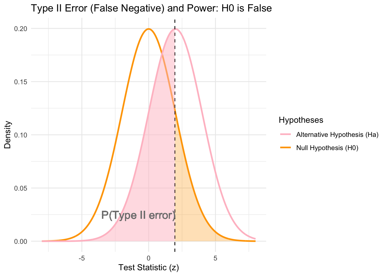
This plot represents the scenario when H_0 is false (i.e., H_a is true; represented by the pink curve). Type II error occurs when H_0 is not rejected. There is the same critical value as before z_{\alpha} (dashed vertical line), separating the rejection and acceptance regions for H_0. The pink shaded area to the left of the critical value represents the probability of Type II error (\beta), which is the probability of failing to reject H_0 when it is false. The power is the probability of correctly rejecting the null hypothesis H_0 when it is false, and so Power = 1-\beta. It measures the test’s ability to detect a true effect or difference.
18 Section 5: Methods to correct for multiple testing
We looked at four methods to correct for multiple testing: Bonferroni, Benjamini-Hochberg (BH), Pocock and O’Brien-Fleming.
18.1 Summary of multiple comparison correction methods
| Method | Uniform bounds | Description |
|---|---|---|
| Bonferroni | Yes | Conservative method that adjusts p-values (or significance levels) uniformly. |
| Pocock | Yes | Uses a uniform significance threshold for all interim analyses to control type I error. |
| Benjamini-Hochberg (BH) | No | Adjusts p-values based on rank to control false discovery rate, allowing more discoveries. |
| O’Brien-Fleming | No | Uses conservative critical values for earlier interim analysis and less conservative values as more data are collected. |
18.2 Details and R code:
Bonferroni and BH procedures with p.adjust()
p_values <- c(0.01, 0.04, 0.03, 0.005,0.03,0.01)  # Example p-values

# Adjust p-values using Bonferroni correction
bonferroni_p <- p.adjust(p_values, method = "bonferroni")
bonferroni_p
[1] 0.06 0.24 0.18 0.03 0.18 0.06# Adjust p-values using Benjamini-Hochberg (BH) procedure
bh_p <- p.adjust(p_values, method = "BH")
bh_p[1] 0.020 0.040 0.036 0.020 0.036 0.020We use the package gsDesign to get critical values for the Pocock’s and O’Brien-Fleming methods:
Template:
gsDesign(
        k = number_interim_analysis,
        test.type = Type_of_test,   #(e.g., 1 = two-sided, 2 = one-sided,..)
        delta = default_effect_size,
        alpha = type_I_error_rate ,
        beta =  type_II_error_rate,
        sfu = boundary_type)
Example:
design_pocock <- gsDesign(
                      k = 10,
                      delta = 0,
                      test.type = 1,
                      alpha = 0.05,
                      beta = 0.2,
                      sfu = "Pocock")

critical_values_pocock = design_pocock$upper$bound
critical_values_pocock
[1] 2.270003 2.270003 2.270003 2.270003 2.270003 2.270003 2.270003 2.270003
[9] 2.270003 2.270003design_OF <- gsDesign(
k = 10,
test.type = 1,
delta = 0,
alpha = 0.05,
beta = 0.2,
sfu = 'OF')
critical_values_OF = design_OF$upper$bound
critical_values_OF [1] 5.695930 4.027631 3.288547 2.847965 2.547297 2.325354 2.152859 2.013815
[9] 1.898643 1.801211