library(tidyverse)
library(infer)11 STAT 201 R Cheatsheet
11.1 Set-up
To be able to run the functions below you need to load the following packages.
Throughout this cheatsheet we will use the Palmer penguin dataset to show examples of code. This dataset is found in the R package palmerpenguins.
library(palmerpenguins)We will focus mostly on the flipper length (mm) of the penguins species Chinstrap and Adelie, and thus will create new data frames called adelie and chinstrap.
adelie <- penguins %>%
  filter(!is.na(flipper_length_mm) &
           species == "Adelie" & !is.na(sex)) %>%
  droplevels() %>%
  dplyr::select(species, flipper_length_mm, sex)

chinstrap <- penguins %>%
  filter(!is.na(flipper_length_mm) &
           species == "Chinstrap" & !is.na(sex)) %>%
  droplevels() %>%
  dplyr::select(species, flipper_length_mm, sex)
Using the penguins_raw dataset, we will also looked at changes in body mass for Gentoo penguins that were captured on Biscoe Island in 2008 and recaptured on the same Island in 2009.
gentoo_mass_diff <- penguins_raw %>%
  filter(Species == "Gentoo penguin (Pygoscelis papua)" &
           Island == "Biscoe" & !is.na("Body Mass (g)")) %>%
  droplevels() %>%
  rename( "ID" = `Individual ID`, "Body_mass_g" = `Body Mass (g)`) %>%
  mutate(Year = as.numeric(paste("20", substring(studyName, 4, 5),
                                 sep = ""))) %>%
  filter(Year == 2008 | Year == 2009) %>%
  filter(duplicated(ID, fromLast = TRUE) | duplicated(ID) ) %>%
  select(ID, Body_mass_g, Sex, Year) %>%
  arrange(ID)

# Check that we have 2 rows (1 per year) per individual
gentoo_mass_diff %>% group_by(ID) %>% count() %>% pull(n) %>% unique()
[1] 211.2 Sampling
11.2.1 rep_sample_n(tbl = , size = , reps = , replace = FALSE)
rep_sample_n() is in the infer package. You will need to run library(infer) to access the function (see set-up section).
Takes a sample from the data frame provided by
tbl =(which may be piped in). If you use%>%, you don’t need to specifytbl.Specify the sample size with
size =.Specify the number of replicates to take with
reps =.Specify if the sample should be taken with replacement (
replace = TRUE) or without replacement (replace = FALSE). The default is without replacement.
resamples <- adelie %>%
  rep_sample_n(size = 20, reps = 1000, replace = FALSE)
head(resamples)
# A tibble: 6 × 4
# Groups: replicate [1]
replicate species flipper_length_mm sex
<int> <fct> <int> <fct>
1 1 Adelie 178 female
2 1 Adelie 190 female
3 1 Adelie 183 female
4 1 Adelie 185 male
5 1 Adelie 192 female
6 1 Adelie 205 male tail(resamples)# A tibble: 6 × 4
# Groups: replicate [1]
replicate species flipper_length_mm sex
<int> <fct> <int> <fct>
1 1000 Adelie 184 male
2 1000 Adelie 199 female
3 1000 Adelie 192 female
4 1000 Adelie 189 female
5 1000 Adelie 187 female
6 1000 Adelie 193 male The object returned, here resamples, has a variable that contains which of the reps replicate the row belongs to and the resampled values.
11.3 Grouping and ungrouping data
11.3.1 group_by(.data, ...)
Groups the data by the argument provided.
res_group <- resamples %>% group_by(replicate)
head(res_group)
# A tibble: 6 × 4
# Groups: replicate [1]
replicate species flipper_length_mm sex
<int> <fct> <int> <fct>
1 1 Adelie 178 female
2 1 Adelie 190 female
3 1 Adelie 183 female
4 1 Adelie 185 male
5 1 Adelie 192 female
6 1 Adelie 205 male Note that resamples was already grouped as rep_sample_n() returns an object grouped by replicate.
11.3.2 ungroup(x, )
Ungroups the data.
res_ungroup <- resamples %>% ungroup()
head(res_ungroup)
# A tibble: 6 × 4
replicate species flipper_length_mm sex
<int> <fct> <int> <fct>
1 1 Adelie 178 female
2 1 Adelie 190 female
3 1 Adelie 183 female
4 1 Adelie 185 male
5 1 Adelie 192 female
6 1 Adelie 205 male Notice the difference between the two. The output of head(res_ungroup) does not have # Groups: replicate [1]
11.4 Calulating statistics
11.4.1 summarize(.data, statistic_value = statistic_function(variable_of_interest))
Calculates statistics on a data frame that may or may not be grouped. It returns one row for each combination of grouping variables.
statistic_value is your name for the statistic
statistic_function is an R function
variable_of_interest is a column in the data frame
resamples %>% summarize(sample_mean = mean(flipper_length_mm))# A tibble: 1,000 × 2
replicate sample_mean
<int> <dbl>
1 1 189.
2 2 190.
3 3 189.
4 4 193.
5 5 192.
6 6 189.
7 7 189.
8 8 192.
9 9 190.
10 10 191.
# ℹ 990 more rows11.5 Bootstrap distributions with the infer package
specify(x, response = )
generate(x, type = "bootstrap", reps = )
calculate(x, stat = )
On the data frame x:
specify()the variable you’re interested inresponse =generate()the bootstrap samples with the specified number ofreps =for each sample, calculates the statistic specified in
stat =which should be one of:- “mean”, “median”, “sum”, “sd”, “prop”, “count”, “diff in means”, “diff in medians”, “diff in props”
median_bootstrap <- adelie %>%
  specify(response = flipper_length_mm) %>%
  generate(type = "bootstrap", reps = 1000) %>%
  calculate(stat = "median")
head(median_bootstrap)
Response: flipper_length_mm (numeric)
# A tibble: 6 × 2
replicate stat
<int> <dbl>
1 1 190.
2 2 191
3 3 190
4 4 190
5 5 190
6 6 190 11.6 Confidence intervals with the infer package
11.6.1 get_ci(x, level = , type ="percentile")
Calculates a confidence interval of the specified level of confidence (level =) on the distribution x.
median_95ci <- median_bootstrap %>%
  get_ci(level = 0.95, type = "percentile")
median_95ci
# A tibble: 1 × 2
lower_ci upper_ci
<dbl> <dbl>
1 189 19111.7 Data visualization: ggplot2
ggplot2 is a flexible and powerful visualization package in R that creates plots by combining different components. It can be used for many types of plots, such as histograms, scatter plots, and line plots. The base function in ggplot2 is ggplot(), which initializes the plot. Additional layers can then be added to specify the details of the plot by using geom_*() functions. geom_*() functions define the type of plot (e.g., geom_histogram() for histograms, geom_point() for scatterplot, geom_boxplot() for boxplot).
ggplot2 uses general functions for titles and axis labels. They are used to customize the plot but don’t define the data visualization itself. You can use them to add titles, and axis labels, and customize other aspects of the plot:
ggtitle(): Adds a main title to the plotxlab(): Labels the x-axisylab(): Labels the y-axisscale_fill_manual(): Colors for categorical variables when plotting. In the context of boxplots, scatter plots, bar charts, or any other plot type, it allows you to control the color aesthetics (e.g., the fill color) for different groups or categories.
11.7.1 ggplot(data = , aes(x = )) + geom_histogram(binwidth = )
Plots a histogram of the data.
Specify the variable on the x-axis with
aes(x = )In
geom_histogram(), specify thebinwidth =or thebins =
median_dist_plot <- median_bootstrap %>%
  ggplot(aes(x = stat)) +
  geom_histogram(bins = 10) +
  ggtitle("Sampling distribution") +
  xlab("Median flipper length (mm)")
median_dist_plot
11.7.2 annotate(geom, "rect", xmin = , xmax = , ymin = , ymax = , fill = , alpha = )
Adds a shaded rectangle to a geom with the specified boundaries (xmin =, xmax =, ymin =, ymax = ), fill colour (fill = ), and transparency level (alpha = ).
Template:
median_dist_plot +
  annotate("rect",
           xmin = median_95ci$lower_ci,
           xmax = median_95ci$upper_ci,
           ymin = 0, ymax = Inf, fill = "deepskyblue",
           alpha = 0.3)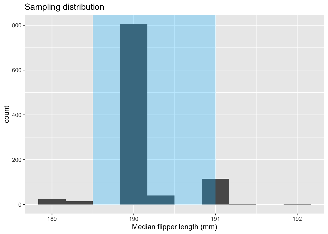
11.8 ggplot(data = , aes(x = )) + geom_boxplot()
Plots a boxplot of the data.
  ggplot(data = penguins, aes(x = species, y = flipper_length_mm, fill = species)) +
  geom_boxplot() +
  ggtitle("Boxplot of Flipper Length by Species") +  # Add a title
  xlab("Species") +  # Label for the x-axis
  ylab("Flipper Length (mm)") + # Label for the y-axis
  scale_fill_manual(values = c("Adelie" = "skyblue", "Chinstrap" = "orange", "Gentoo" = "#2e8b57"))  # Custom colors for each species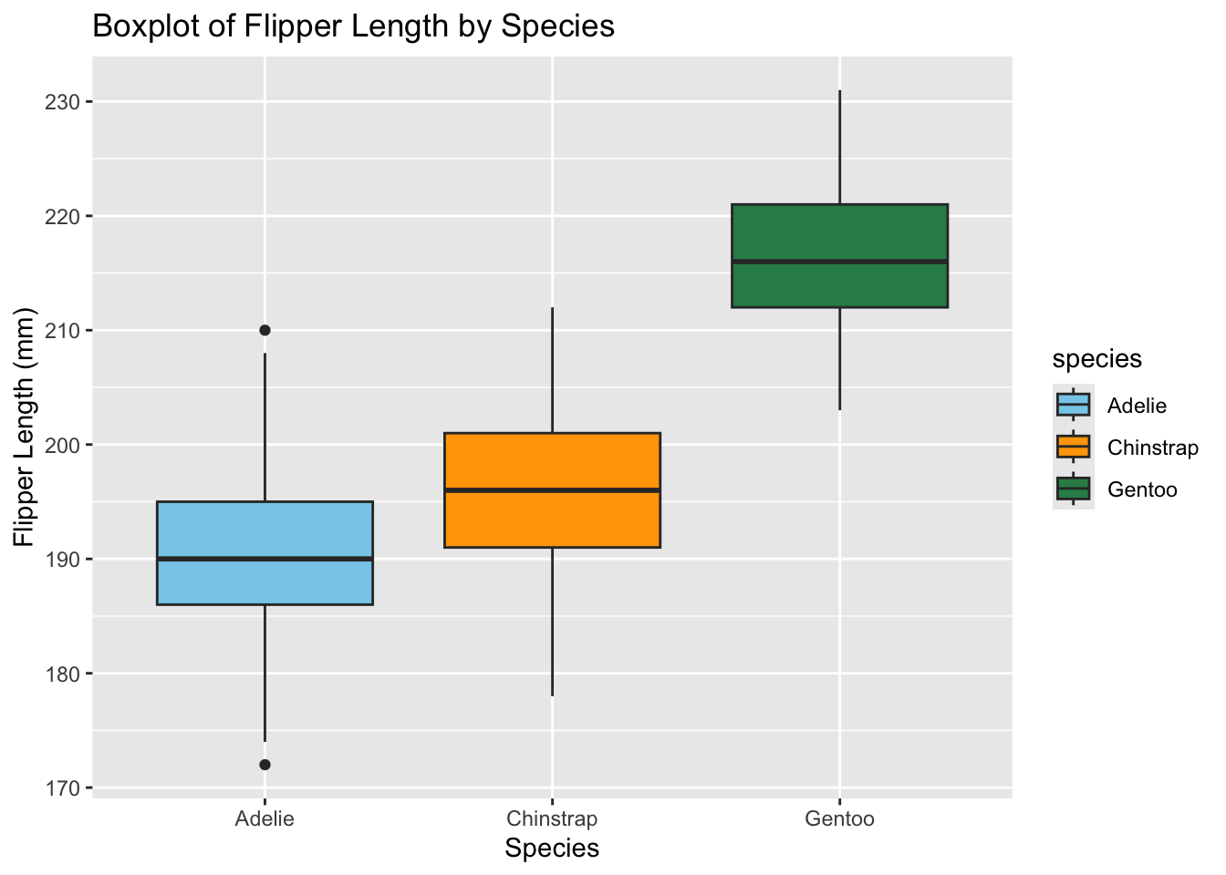
11.9 Calculating quantiles
11.9.1 quantile(x, probs = )
Calculates the sample quantile on the data x corresponding to the given probability probs.
median_bootstrap %>% pull(stat) %>% quantile(0.05) 5%
190 11.10 Normal and t-distribution functions
11.10.1 qnorm(p, mean = , sd = )
Calculates a quantile on the normal distribution with specified mean (mean =) and standard deviation (sd =) where the proportion p of the distribution is less than the quantile. The default is mean = 0 and sd = 1 (i.e. the standard normal).
qnorm(0.25, 57, 54.4)[1] 20.3077611.10.2 dnorm(x, mean=, sd =)
Calculates the probability density function (PDF) for the normal distribution with mean mean and standard deviation sd. It returns the density of the normal distribution at a x. The default values for mu is 0 and sd is 1.
dnorm(0.25, mean = 1, sd=1)[1] 0.301137411.10.3 pnorm(x, mean=, sd =)
Calculates the cumulative distribution function for the normal distribution with mean mean and standard deviation sd. The default is a standard normal distribution (mean is 0 and sd is 1). It returns the probability that a normally distributed random variable is less than or equal to x.
pnorm(0.25, mean = 1, sd=1)[1] 0.2266274pnorm and qnorm take a lower.tail argument, for which default value is TRUE. It controls whether the function computes probabilities or quantiles for the lower (TRUE) or upper tail (FALSE) of the distribution.
pnorm(2, mean = 0, sd = 1) # P(X <= 2) for a standard normal distribution[1] 0.9772499pnorm(2, mean = 0, sd = 1, lower.tail = FALSE) # P(X > 2) for a standard normal distribution[1] 0.0227501311.10.4 qt(p, df = )
Calculates a quantile on the t-distribution with specified degrees of freedom (df =) where the proportion p of the distribution is less than the quantile.
qt(0.25, 23)[1] -0.685306311.10.5 dt(x, df = )
Calculates the density of the t-distribution with specified degrees of freedom (df =) at observation x. It gives the likelihood of a value occurring at x in a t-distribution, as opposed to the cumulative probability (see below).
dt(0.25, 23)[1] 0.381986811.10.6 pt(x, df = )
Calculates the cumulative distribution function (CDF) of the t-distribution. It is used when we want to determine the probability that a value drawn from a t-distribution with df degrees of freedom is less than or equal to x.
pt(0.25, 23)[1] 0.5975966pt and qt take a lower.tail argument, for which default value is TRUE. It controls whether the function computes probabilities or quantiles for the lower (TRUE) or upper tail (FALSE) of the distribution.
pt(2, df = 23) # P(X <= 2) for a t-distribution with 2 degrees of freedom[1] 0.9712777pt(2, df = 23, lower.tail = FALSE) # P(X > 2) for a t-distribution with 2 degrees of freedom[1] 0.0287222711.11 Hypothesis testing
11.12 Method 1: Simulation
Hypothesis testing with the infer package:
specify()specifies the variable that you are interested in, and sometimes (e.g. independent two-sample tests) a formula that describes how the variable is groupedhypothesise(null)states the null hypothesis, which should be one of:hypothesise(null = "point", mu = mu_0)hypothesise(null = "independence")hypothesise(null = "paired independence")
generate(type = ... , rep = ...)generates the resamplescalculate(stat = ...)calculates the statistic you are interested in for each re-sampleget_p_value()calculates the p-value of the test.
11.12.1 Bootstrap hypothesis testing (resampling with replacement)
When using bootstrap hypothesis testing, we set the type argument of generate() to "bootstrap".
Test whether a single parameter (i.e., proportion, mean, median, sigma) differs from a hypothesised value
Example: mean
hypothesise(null = "point", mu = mu_0) tests if the population mean is equal to mu_0.
mu_0 = 190
# Create null distribution
mean_null <- adelie %>%
  specify(response = flipper_length_mm) %>% #  Step 1: Specify model
  hypothesise(null = "point", mu = mu_0) %>%  # Step 2: Set null hypothesis
  generate(type = "bootstrap", reps = 1000) %>% # Step 3: Generate null distribution
  calculate(stat = "mean")  # Step 4: Calculate test statistic

# Get p-value
get_p_value(mean_null, obs_stat = mean(adelie$flipper_length_mm), direction = "both")  # Step 5: Calculate the p value
# A tibble: 1 × 1
p_value
<dbl>
1 0.826Example: median
hypothesise(null = "point", med = med_0) tests if the population median is equal to mu_0.
med_0 = 189
# Create null distribution
median_null <- adelie %>%
  specify(response = flipper_length_mm) %>% #  Step 1: Specify model
  hypothesise(null = "point", med = med_0) %>%  # Step 2: Set null hypothesis
  generate(type = "bootstrap", reps = 1000) %>% # Step 3: Generate null distribution
  calculate(stat = "median")  # Step 4: Calculate test statistic

# Get p-value
get_p_value(median_null, obs_stat = median(adelie$flipper_length_mm), direction = "both")  # Step 5: Calculate the p value
# A tibble: 1 × 1
p_value
<dbl>
1 0.232Test whether a set of paired population differ
hypothesise(null = "paired independence") should be used when testing paired data, where each observation in one sample has a corresponding observation in another sample.
11.12.2 Permutation resampling (sample without replacement, like shuffling)
When using permutation hypothesis testing, we set the type argument of generate() to "permute".
hypothesise(null = "independence") should be used to test whether two groups are independent, meaning there is no association or relationship between them in the population (e.g., flipper length between two different penguin species).
In addition:
specify(formula)needs a formula of the form y \sim x wherexis the response (e.g., flipper_length_mm) andythe explanatory variable (e.g., species). Permutation resampling won’t work withinferif the explanatory variable is not specified since permutation resampling is commonly used to test for independence or equality between two groups.
Example: difference in median
We will look at where there is a difference in the median flipper length (mm) between female and male adelin penguins.
obs_diff_in_medians <-
    adelie  %>%
    specify(formula = flipper_length_mm ~ sex) %>%
    calculate(stat = "diff in medians", order = c("female", "male"))

# get p-value
    adelie %>%
    specify(formula = flipper_length_mm ~ sex) %>% # Step 1: Specify model
    hypothesize(null = "independence") %>%  # Step 2: Set null hypothesis
    generate(reps = 1000, type = "permute")  %>% #  Step 3: Generate null distribution
    calculate(stat = "diff in medians", order = c("female", "male"))%>%  # Step 4: Calculate test statistic
    get_p_value(obs_stat =  obs_diff_in_medians, direction = "both") # Step 5: Calculate the p value
# A tibble: 1 × 1
p_value
<dbl>
1 011.13 Method 2: Theory-based hypothesis testing
Theory-based hypothesis tests require assumptions on the data.
11.13.1 Proportions (categorical): Z-tests
For one group:
The test statistic of the z-test is:
Z = \frac{\hat{p} - p_0}{\sqrt{\frac{p_0 (1 - p_0)}{n}}},
Z \sim N(0, 1), (approx.)
where \hat{p} is the sample proportion, p_0 is the hypothesized proportion value, and n is the sample size.
Example: we think that the proportion p of female adelie penguins is greater than p_0 = 0.5. It can be written as follows: H_0: p = 0.5, H_1: p > 0.5
# Hypothesized proportion
adelie_p0_f <- 0.5
# Observed proportion of females
adelie_prop_f <-  mean(adelie$sex == "female")
# Estimated standard error
adelie_prop_f_se <- sqrt(adelie_p0_f * (1 - adelie_p0_f) / nrow(adelie))

# Calculate the p-value
pnorm(adelie_prop_f, 0.5, adelie_prop_f_se, lower.tail = FALSE)
[1] 0.5Difference between two groups:
The test statistic used when comparing the proportion from two independent populations is:
Z = \frac{(\hat{p}_1 - \hat{p}_2) - \Delta_0}{\sqrt{\hat{p}(1 - \hat{p})\left(\frac{1}{n_1} + \frac{1}{n_2}\right)}},
Z \sim N(0, 1), (approx.)
where \hat{p}_1 is the sample proportion of sample 1, \hat{p}_2 is the sample proportion of sample 2, \hat{p} is the sample proportion of for both samples combined, \Delta_0 is the hypothesized difference, n_1 is the size of sample 1, and n_2 is the size of sample 2.
Example:
We want to test whether there is a difference in proportion of flipper longer than 200 mm between species.
# Calculate proportions of flipper length > 200 for Adelie and Chinstrap
prop_adelie <- mean(adelie$flipper_length_mm > 200)
prop_chinstrap <- mean(chinstrap$flipper_length_mm > 200)
prop_both <- mean(c(chinstrap$flipper_length_mm > 200, adelie$flipper_length_mm > 200))

# Standard error of the difference in proportions
std_error_diff <- sqrt((prop_both * (1 - prop_both)) *
                         (1/nrow(adelie) + 1/nrow(chinstrap)))

# Z-score for the difference in proportions
z_score <- (prop_chinstrap - prop_adelie) / std_error_diff

# P-value for the two-tailed test
p_value <- 2 * pnorm(abs(z_score), lower.tail = FALSE)
11.13.2 Means: t-test and ANOVA
One group: one sample t-test
The test statistic to test whether the population mean differ from a hypothesized value is:
- T = \frac{(\bar{X} - \mu_0)}{s/\sqrt{n}},
- T \sim t_{n-1}, (approx.)
where \bar{X} is the sample mean, \mu_0 is the hypothesized mean, s is the sample standard deviation, n is the sample size, and n-1 is the degrees of freedom of the t-distribution.
Example: we want to test if the average flipper length of adelie penguins is different from 190.
mu0 <- 190

# Calculate sample statistics
sample_mean <- mean(adelie$flipper_length_mm)
sample_sd <- sd(adelie$flipper_length_mm)

# Calculate the t-statistic
t_statistic <- (sample_mean - mu0) / (sample_sd / sqrt(nrow(adelie)))

# Calculate the p-value (two-tailed) using pt()
2 * pt(-abs(t_statistic), df = (nrow(adelie) - 1))
[1] 0.8493036Alternatively we can use the t.test(x,...) function as follows:
x: data for the variable of interest (e.g., flipper_length_mm)alternative: the direction of the alternative. It can be eithertwo.sided,lessorgreater.
t.test(x = adelie$flipper_length_mm,
       mu = 190,
       alternative = "two.sided")
Difference between two independent groups: two-sample t-test
The test statistics to compare the mean of two independent population is:
- T = \frac{\bar{X}_1 - \bar{X}_2 - \Delta_0}{\sqrt{\frac{s_1^2}{n_1} + \frac{s_2^2}{n_2}}},
- T \sim t_{\min(n_1 - 1, n_2 - 1)}, (approx.)
where \bar{X}_1 is the mean of sample 1, \bar{X}_2 is the mean of sample 2, \Delta_0 is the hypothesized difference between the mean of two population under the null, s_1 is the standard deviation of sample 1, s_2 is the standard deviation of sample 2, n_1 is the size of sample 1, n_2 is the size of sample 2, and \min(n_1 - 1, n_2 - 1) is the degrees of freedom of the t-distribution. Note that other, and better ways to calculate the degrees of freedom are often used. We use \min(n_1 - 1, n_2 - 1) for simplicity.
Example: we want to test whether there is significant difference between the average flipper length of difference penguin species.
# Compute the means for both groups
mean_adelie <- mean(adelie$flipper_length_mm)
mean_chinstrap <- mean(chinstrap$flipper_length_mm)

# Compute sample sd for both groups
sd_adelie <- sd(adelie$flipper_length_mm)
sd_chinstrap <- sd(chinstrap$flipper_length_mm)
# Calculate the pooled standard error
pooled_se <- sqrt((sd_adelie^2 / nrow(adelie)) + (sd_chinstrap^2 / nrow(chinstrap)))
# Calculate the t-statistic for the difference in means
t_statistic <- (mean_adelie - mean_chinstrap) / pooled_se
# Calculate the two-tailed p-value using pt()
2 * pt(-abs(t_statistic), df = min( nrow(adelie) - 1, nrow(chinstrap) - 1))[1] 4.143797e-07Alternatively, we can use the t.test() function, where:
x: variable for group 1y: variable for group 2mu: hypothesized difference. The default is0(i.e. there is no difference between the two populations).alternative: direction of the alternative hypothesis. The options are “two.sided”, “less”, “greater”.var.equal: the method we learned in class assumes that the variance is equal in the two population, thus this argument is set toTRUE. But one useFALSEif there is evidence that the variance is unequal.
t.test(adelie$flipper_length_mm,
       chinstrap$flipper_length_mm,
       alternative = "two.sided",
       var.equal = TRUE)
    Two Sample t-test

data:  adelie$flipper_length_mm and chinstrap$flipper_length_mm
t = -5.7979, df = 212, p-value = 2.413e-08
alternative hypothesis: true difference in means is not equal to 0
95 percent confidence interval:
 -7.66579 -3.77579
sample estimates:
mean of x mean of y
190.1027 195.8235 t.test()uses a different approximation of the degree of freedom df than \min(n_1 - 1, n_2 - 1), which explains the different result. The use of \min(n_1 - 1, n_2 - 1) is a “conservative” estimate of the degrees of freedom. The function t.test() uses df = n_1 + n_2 - 2.
11.13.3 Difference between paired groups: paired-sample t-test
The test statistic to compare the mean of two paired populations is:
- T = \frac{\bar{d} - \Delta_0}{\frac{s_d}{\sqrt{n}}},
- T \sim t_{n - 1}, (approx.)
where \bar{d} is the mean difference in paired values from both samples, \Delta_0 is the hypothesized difference between the paired population under the null, s_d is the standard deviation of the differences in paired values from both samples, and n - 1 is the degree of freedom of the t-distribution.
Example:
Using the t.test() function
x: variable for sample 1y: variable for sample 2mu: hypothesized difference. The default is0(i.e. there is no difference between the two populations).alternative: direction of the alternative hypothesis. The options are “two.sided”, “less”, “greater”.paired: set toTRUEfor paired t-test
Test whether the body mass of Gentoo penguins on Biscoe Island differ between 2008 and 2009.
mass_2008 <- gentoo_mass_diff %>% filter(Year == 2008)
mass_2009 <- gentoo_mass_diff %>% filter(Year == 2009)

t.test(mass_2008$Body_mass_g, mass_2009$Body_mass_g,
       alternative = "two.sided", paired = TRUE)
    Paired t-test

data:  mass_2008$Body_mass_g and mass_2009$Body_mass_g
t = -0.87943, df = 15, p-value = 0.393
alternative hypothesis: true mean difference is not equal to 0
95 percent confidence interval:
 -385.1638  160.1638
sample estimates:
mean difference
         -112.5
11.13.4 Difference between three or more independent groups ANOVA
One-way ANOVA
11.14 aov()
Fits an ANOVA to the data.
one_way_anova <- aov(flipper_length_mm ~ species, data = penguins)
summary(one_way_anova)
Df Sum Sq Mean Sq F value Pr(>F)
species 2 52473 26237 594.8 <2e-16 ***
Residuals 339 14953 44
---
Signif. codes: 0 '***' 0.001 '**' 0.01 '*' 0.05 '.' 0.1 ' ' 1
2 observations deleted due to missingnessaov() takes formula as an argument (of usual form y \sim x). This should specify the response of interest (e.g., flipper_length_mm) and the explanatory variable (e.g., species). The function summary returns the following:
Df: Degrees of freedom for the factor (species) and residuals.Sum Sq: The sum of squares for species and residuals.Mean Sq: The mean sum of squares, calculated by dividing the sum of squares by the degrees of freedom.F value: The F-statistic for the factor (here species). It tests whether the means of species differ significantly).Pr(>F): p-value.
11.15 Multiple testing
11.15.1 p.adjust(p, method = "")
Provides a numeric vector of corrected p-values (of the same length as p, with names copied from p).
Specify
p, a numeric vector of p-valuesSpecify the method that you want to use to adjust p-values in the argument
methodwhich should be one of:- “holm”, “hochberg”, “hommel”, “bonferroni”, “BH”, “BY”, “fdr”, “none”.
# Create vector of p-values
p_values = c(0.001,0.34,0.21,0.012,0.4,0.01)
pval_bonf <- p.adjust(p_values, method = "bonferroni")