Lecture 6: Factors

October 9, 2025

Modified

October 13, 2026

Lecture Slides

Lecture 6 Slides

Video Lecture

From today’s class, students are anticipated to be able to:

Reorder levels within factors according to various principles

Set-up

Throughout this lecture, we will be using functions from the following packages:

library(tidyverse) #also loads forcats!
library(palmerpenguins)
library(gapminder)

Factors

“There is no other object that creates as much trouble as factors.” - Patrick Burns, “The R Inferno”.

In R, we use factors to represent categorical variables: variables that take on a fixed number of known values (i.e. levels). For example, in the penguins data set, species is a factor with three levels: “Adelie”, “Chinstrap”, and “Gentoo”. We can see this by looking at the str() (structure) of the tibble:

str(penguins)

tibble [344 × 8] (S3: tbl_df/tbl/data.frame)
 $ species          : Factor w/ 3 levels "Adelie","Chinstrap",..: 1 1 1 1 1 1 1 1 1 1 ...
 $ island           : Factor w/ 3 levels "Biscoe","Dream",..: 3 3 3 3 3 3 3 3 3 3 ...
 $ bill_length_mm   : num [1:344] 39.1 39.5 40.3 NA 36.7 39.3 38.9 39.2 34.1 42 ...
 $ bill_depth_mm    : num [1:344] 18.7 17.4 18 NA 19.3 20.6 17.8 19.6 18.1 20.2 ...
 $ flipper_length_mm: int [1:344] 181 186 195 NA 193 190 181 195 193 190 ...
 $ body_mass_g      : int [1:344] 3750 3800 3250 NA 3450 3650 3625 4675 3475 4250 ...
 $ sex              : Factor w/ 2 levels "female","male": 2 1 1 NA 1 2 1 2 NA NA ...
 $ year             : int [1:344] 2007 2007 2007 2007 2007 2007 2007 2007 2007 2007 ...

or we can explicitly look at the class and levels of the variable of interest by:

class(penguins$species)

[1] "factor"

levels(penguins$species)

[1] "Adelie"    "Chinstrap" "Gentoo"

Under the hood, R stores a factor with (say) 3 levels as a numeric vector containing integers between 1 and 3, paired with a character vector of length 3 that identifies the mapping between the numbers 1, 2, and 3 and the levels.

This is not immediately obvious, because R will print factors using the character string levels rather than the numbers that it stores:

set.seed(100) #make reproducible (more on this later)

penguins %>% 
  slice_sample(n=10) %>% #take 10 random rows
  pull(species) #output the species only

 [1] Gentoo    Adelie    Gentoo    Adelie    Chinstrap Chinstrap Adelie   
 [8] Adelie    Gentoo    Chinstrap
Levels: Adelie Chinstrap Gentoo

This dual nature of factors creates a whole slew of hidden traps and headaches, especially for new R users!

Caution

Sometimes factors are coded (i.e., written) in the data as integers. Without explicitly telling R, R will assume any numeric data are just regular old numbers.

Always ensure that factors are explicit in your code!

For example, suppose in the penguins data set than instead of their names, species had levels “1”, “2”, and “3’ where”1” could represent Gentoo, “2” Adelie, and 3 “Chinstrap” penguins. So, instead of having the names of penguin species as strings, they are coded as numeric values.

penguins2 <- penguins %>%
  mutate(species = recode(species, "Gentoo" = 1, "Adelie" = 2, "Chinstrap" = 3))

str(penguins2)

tibble [344 × 8] (S3: tbl_df/tbl/data.frame)
 $ species          : num [1:344] 2 2 2 2 2 2 2 2 2 2 ...
 $ island           : Factor w/ 3 levels "Biscoe","Dream",..: 3 3 3 3 3 3 3 3 3 3 ...
 $ bill_length_mm   : num [1:344] 39.1 39.5 40.3 NA 36.7 39.3 38.9 39.2 34.1 42 ...
 $ bill_depth_mm    : num [1:344] 18.7 17.4 18 NA 19.3 20.6 17.8 19.6 18.1 20.2 ...
 $ flipper_length_mm: int [1:344] 181 186 195 NA 193 190 181 195 193 190 ...
 $ body_mass_g      : int [1:344] 3750 3800 3250 NA 3450 3650 3625 4675 3475 4250 ...
 $ sex              : Factor w/ 2 levels "female","male": 2 1 1 NA 1 2 1 2 NA NA ...
 $ year             : int [1:344] 2007 2007 2007 2007 2007 2007 2007 2007 2007 2007 ...

We see here that R assumes that species is a numeric variable, not a categorical variable. To ensure R knows that species is categorical, we can use:

penguins2 <- penguins2 %>% #overwrite existing tibble
  mutate(species = as.factor(species)) #overwrite species to be a factor using as.factor

str(penguins2)

tibble [344 × 8] (S3: tbl_df/tbl/data.frame)
 $ species          : Factor w/ 3 levels "1","2","3": 2 2 2 2 2 2 2 2 2 2 ...
 $ island           : Factor w/ 3 levels "Biscoe","Dream",..: 3 3 3 3 3 3 3 3 3 3 ...
 $ bill_length_mm   : num [1:344] 39.1 39.5 40.3 NA 36.7 39.3 38.9 39.2 34.1 42 ...
 $ bill_depth_mm    : num [1:344] 18.7 17.4 18 NA 19.3 20.6 17.8 19.6 18.1 20.2 ...
 $ flipper_length_mm: int [1:344] 181 186 195 NA 193 190 181 195 193 190 ...
 $ body_mass_g      : int [1:344] 3750 3800 3250 NA 3450 3650 3625 4675 3475 4250 ...
 $ sex              : Factor w/ 2 levels "female","male": 2 1 1 NA 1 2 1 2 NA NA ...
 $ year             : int [1:344] 2007 2007 2007 2007 2007 2007 2007 2007 2007 2007 ...

Now we see that species is a factor with three levels!

Nevertheless, factors are important and worth the pain. Many functions throughout the R landscape expect categorical variables to be coded as factors. For example, when making plots in either ggplot2 or in base R, we need factors in order to map categorical variables to aesthetic elements like colour.

To make our lives easier, we will work with factors through the forcats package loaded as part of the tidyverse.

Reordering Factor Levels

By default, factors are ordered alphabetically or numerically. However, in many cases factors have a logical ordering they should follow. For example, you may have an education variable dictating the level of schooling a student is currently in (i.e., elementary, secondary, post-secondary, graduate). It is natural to order the factor in this way. In other cases, you may just want to reorder the levels of a factor so that it plots a certain way. Reordering data can be useful for both data visualization and model fitting.

To see the current ordering of a factor variable, we can call levels().

levels(penguins$species)

[1] "Adelie"    "Chinstrap" "Gentoo"

We see here, the levels of the factor are ordered alphabetically.

Reordering Levels of a Factors Manually

There are many ways to reorder the levels of a factor in R. To reorder the levels of the factor, we can use built in R functions such as ordered():

penguins3 <- penguins %>%
  mutate(species = ordered(species, levels = c("Gentoo", "Chinstrap", "Adelie"))) #change species to an ordered factor with the specified ordering

levels(penguins3$species) #see the levels of species

[1] "Gentoo"    "Chinstrap" "Adelie"

Now, when we call str() on the penguins data, we see that the factor is explicitly ordered, with out new ordering:

str(penguins3)

tibble [344 × 8] (S3: tbl_df/tbl/data.frame)
 $ species          : Ord.factor w/ 3 levels "Gentoo"<"Chinstrap"<..: 3 3 3 3 3 3 3 3 3 3 ...
 $ island           : Factor w/ 3 levels "Biscoe","Dream",..: 3 3 3 3 3 3 3 3 3 3 ...
 $ bill_length_mm   : num [1:344] 39.1 39.5 40.3 NA 36.7 39.3 38.9 39.2 34.1 42 ...
 $ bill_depth_mm    : num [1:344] 18.7 17.4 18 NA 19.3 20.6 17.8 19.6 18.1 20.2 ...
 $ flipper_length_mm: int [1:344] 181 186 195 NA 193 190 181 195 193 190 ...
 $ body_mass_g      : int [1:344] 3750 3800 3250 NA 3450 3650 3625 4675 3475 4250 ...
 $ sex              : Factor w/ 2 levels "female","male": 2 1 1 NA 1 2 1 2 NA NA ...
 $ year             : int [1:344] 2007 2007 2007 2007 2007 2007 2007 2007 2007 2007 ...

Reordering Levels of a Factors Based on a Condition Using `forcats`

Perhaps we want to reorder levels based on some condition, perhaps the ordering levels by frequency, or perhaps by the another summary statistic (which could be useful for effective data visualization!). We can easily do so using the forcats package. Let’s look again at the original penguins data set and look at the frequency of each species using ggplot:

ggplot(penguins, aes(x = species, fill = species)) + #use species variable (no y needed)
  geom_bar() + #draw a bar chart 
  theme(legend.position = "none")  + #remove redundant legend
  xlab("Species") + #add x axis label
  ylab("Count") + # add y axis label
  ggtitle("Penguin Species Frequencies") #add a title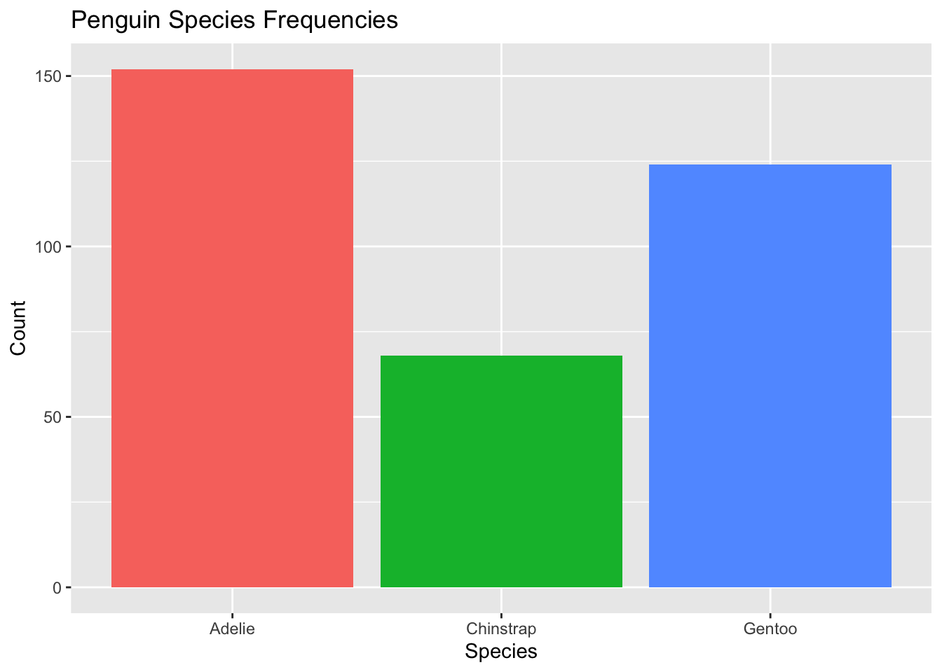

This data visualization is fine. But there’s one step we can do to make it even better: order bars by largest to smallest (or smallest to largest) so readers can easily spot which species is the most common. This is especially useful when the number of levels is large!

We can do this in two ways: edit the original tibble to have new factor ordering, or order the factors directly in the ggplot2 call so that the original tibble isn’t overwritted. We will show both ways. We will use the forcats package in both examples.

Option A: Reorder Tibble Directly

To reorder the factor levels according to the frequency in the tibble, we can use fct_reorder():

penguins4 <- penguins %>% #initialize a new dataset 
  mutate(species = fct_infreq(species))

levels(penguins4$species)

[1] "Adelie"    "Gentoo"    "Chinstrap"

We see the ordering is Adelie, Gentoo, and then Chinstrap. If you look at the previous plot, you’ll see that these are ordered from smallest to largest frequencies. The original ordering was alphabetical.

To order from smallest to largest, we had fct_rev() to the chain:

penguins4 <- penguins %>% #initialize a new dataset 
  mutate(species = species %>%
           fct_infreq() %>%
           fct_rev())


levels(penguins4$species)

[1] "Chinstrap" "Gentoo"    "Adelie"

Now the levels are reversed!

We can then plot our data using penguins4:

ggplot(penguins4, aes(x = species, fill = species)) + #use species variable (no y needed)
  geom_bar() + #draw a bar chart 
  theme(legend.position = "none")  + #remove redundant legend  
  xlab("Species") + #add x axis label
  ylab("Count") + # add y axis label
  ggtitle("Penguin Species Frequencies") #add a title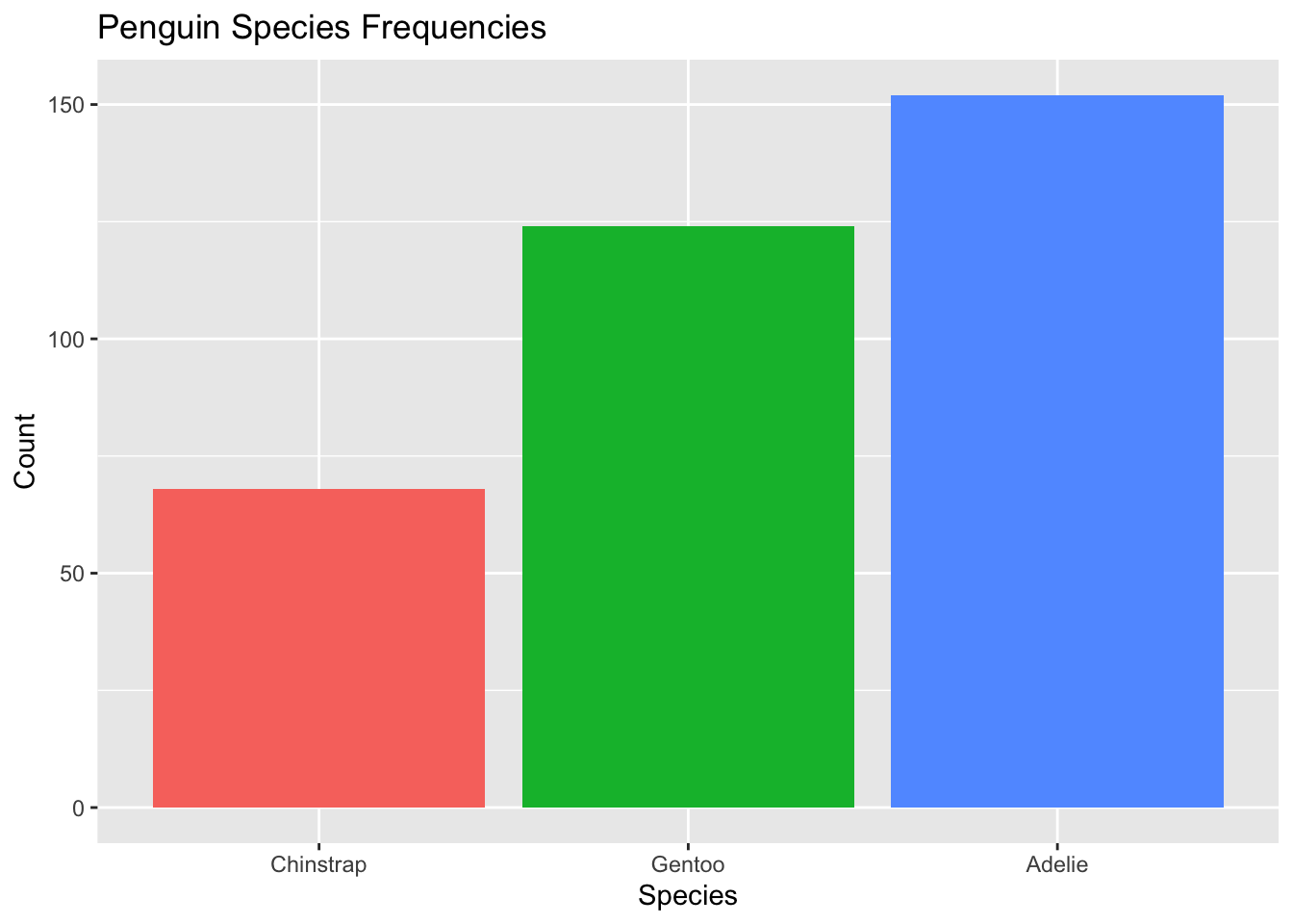

Of course, an even better visualization would involve flipping the axes:

ggplot(penguins4, aes(x = species, fill = species)) + #use species variable (no y needed)
  geom_bar() + #draw a bar chart 
  theme(legend.position = "none")  + #remove redundant legend  
  xlab("Species") + #add x axis label
  ylab("Count") + # add y axis label
  ggtitle("Penguin Species Frequencies") + #add a title
  coord_flip()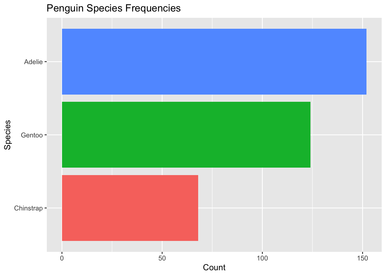

Note

It may look like they are ordered from largest to smallest, but they are actually ordered from smallest to largest. When flipped, ggplot puts the first level on the bottom.

Option B: Reorder the Factor in the ggplot Call

We can do these steps directly in ggplot without overwriting or making a new tibble!

penguins %>% #this is the original data frame with alphabetical ordering
  mutate(species = species %>%
           fct_infreq() %>% #order by frequency
           fct_rev()) %>%  #reverse ordering
  ggplot( aes(x = species, fill = species)) + #no longer specify the data set in ggplot() as this is passed in by the pipe %>%
    geom_bar() + 
    theme(legend.position = "none")  +
    xlab("Species") + 
    ylab("Count") + 
    ggtitle("Penguin Species Frequencies") + 
    coord_flip()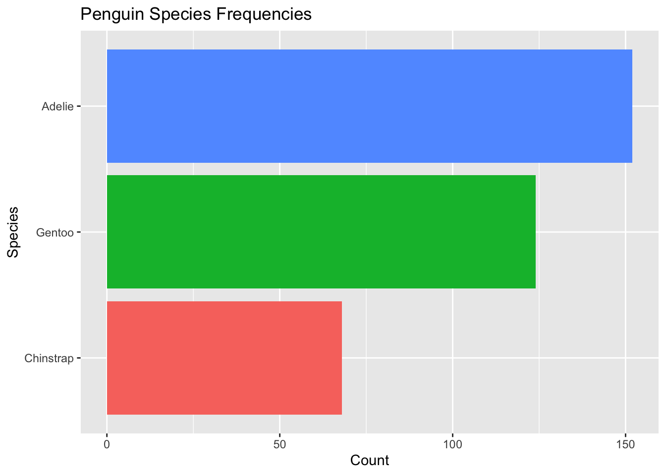

We get the exact same plot with a single chunk of code! And, the original tibble penguins remains unchanged with the alphabetical ordering of the species factors.

levels(penguins$species)

[1] "Adelie"    "Chinstrap" "Gentoo"

Exercise

The gapminder dataset contains information on GDP per capita (gdpPercap) by country. Add to the following ggplot to visualize the GDP per capita, ordered by GDP per capita, for countries in Asia in 2007. Copy the code block to edit and run it in R.

library(gapminder)
library(tidyverse)

gapminder %>%
  filter( ) %>% #FILL THIS IN: filter by countries in Asia
  mutate() %>% #FILL THIS IN: change ordering of country by gdpPercap
  ggplot(aes(country, gdpPercap)) + 
    geom_point() + 
    coord_flip() + 
    scale_y_continuous("GDP per Capita, 2007", labels = scales::dollar_format()) + 
    xlab("Country")

Answer below! No peaking until you’ve attempted this problem!

gapminder %>%
  filter(continent == "Asia", year == 2007) %>% #filter by countries in Asia
  mutate(country = fct_reorder(country, gdpPercap)) %>% #change ordering of country by gdpPercap
  ggplot(aes(country, gdpPercap)) + 
    geom_point() + 
    coord_flip() + 
    scale_y_continuous("GDP per Capita, 2007", labels = scales::dollar_format()) + 
    xlab("Country")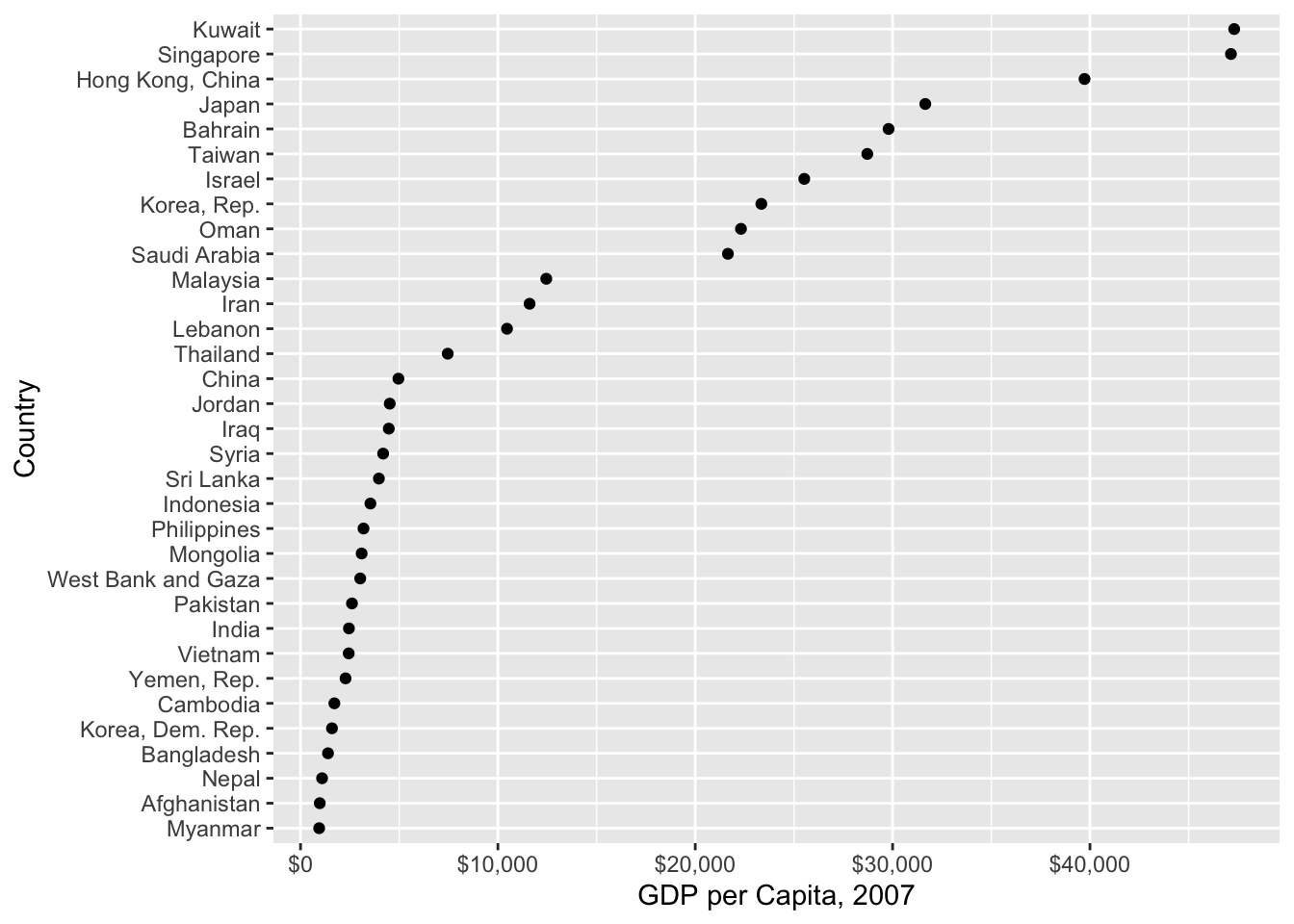

Expanding Factor Levels

Perhaps we may want to visualize that in our data set, there are no Emperor or King penguins. To do so, we can add “Emperor” and “King” as possible factor levels for species in our penguins data set. We do so by fct_expand()

penguins %>% #this is the original data frame with alphabetical ordering
  mutate(species = species %>%
           fct_expand("King", "Emperor") %>% #NEW: expand levels to include king and emperor
           fct_infreq() %>% 
           fct_rev()
           ) %>%  
  ggplot( aes(x = species, fill = species)) + 
    geom_bar() + 
    theme(legend.position = "none")  +
    xlab("Species") + 
    ylab("Count") + 
    ggtitle("Penguin Species Frequencies") + 
    coord_flip() + 
    scale_x_discrete(drop = FALSE) #NEW: do not drop empty factor levels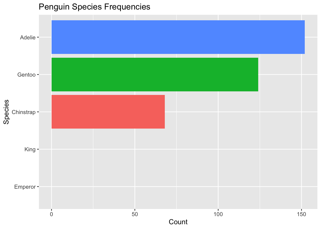

Now we add to the visualization that there were no King or Emperor penguins collected in the data.

Removing Factor Levels

Let’s suppose we were only interested in comparing Adelie and Chinstrap penguins. We could drop the Gentoo level using forcats by:

penguins_no_gentoo <- penguins %>%
  filter(species %in% c("Adelie", "Chinstrap")) %>%
  droplevels()

levels(penguins_no_gentoo$species)

[1] "Adelie"    "Chinstrap"

We can also do this along with the ggplot call by:

penguins %>% #this is the original data frame with alphabetical ordering
  mutate(species = species %>%

           fct_infreq() %>% 
           fct_rev()
           ) %>%  
  filter(species %in% c("Adelie", "Chinstrap")) %>% #NEW: filter only these species
  droplevels() %>% #NEW: drop if not adelie or chinstrap species
  ggplot( aes(x = species, fill = species)) + 
    geom_bar() + 
    theme(legend.position = "none")  +
    xlab("Species") + 
    ylab("Count") + 
    ggtitle("Penguin Species Frequencies") + 
    coord_flip() + 
    scale_x_discrete(drop = FALSE) #NEW: do not drop empty factor levels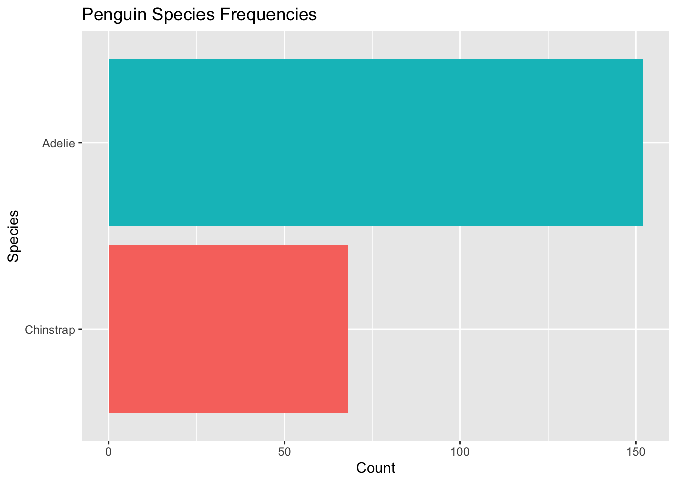

Factors with many levels

Some categorical variables, like birthplace, can have a lot of unique levels.

Consider the case where we have data on 100 individuals with 30 different birthplaces. If we tried to analyze the relationship between birthplace and another variable (say, income), we may run into issues where we do not have enough data in some groups to identify meaningful differences between birthplaces.

There is no universally agreed upon rule as to what constitutes having “too many levels” in a categorical variable, as it often depends on the method(s) being used. Some statisticians argue that you must have >10 observations per level (in our example, this means having 10 or more people in each birthplace)

So… how can you overcome this issue?

Reduce the number of levels, for example:

Use domain knowledge to combine similar levels
Group categories with low frequency together
Use a statistical method to combine similar levels

(Advanced) Use a regularization technique
(Advanced: for hierarchical data) Use the levels as a random effect

Discussion: Race and Ethnicity in Data Analysis

Variables related to race and ethnicity are often collected for studies involving human data.

Definition

Race: a group of people who are arbitrarily categorized according to common physical characteristics, regardless of language, culture or nationality, as per Statistics Canada.

Ethnicity: the shared cultural, linguistic or religious characteristics of a group of people having a common history, heritage or ancestry. While these terms are often used interchangeably, there is a distinct difference which we emphasize here.

There are a lot of unique races and ethnicities that one can collect information on. Oftentimes, these categories are coarsened to have a more reasonable number of possible levels. However, doing so can omit complex racial and ethnic identities which are grouped into broader categories. Further, coarsening the levels may also not acknowledge the unique lived experiences of smaller or mixed-race identities. Such simplifications may lead marginalized groups to be underrepresented in studies, furthering the feeling of invisibility and a lack of belonging.

Discussion

In Canada, Métis have typically been recognized as a “mixed-descent identity” in studies source. How might this affect the Métis population?

For a summary on how Indigenous Peoples were represented in the Canadian Census from 1870 to 2021, see this paper.

Discussion

When plotting or creating tables of demographic variables, an ordering needs to be decided on.

White or Caucasian is frequently shown at the top of tables listing race and ethnicity, and is typically used as a reference group to which other groups are compared source. Placing White at the top of a table or treating it as a reference category can reinforce ideas of white supremacy, stemming from Colonization.

There have been ongoing discussions on how to appropriately include considerations of race and ethnicity into studies, including a guide for researchers in British Columbia..

Use your best judgement, and consider these impacts when handling data on race and ethnicity.
Consider consulting with Indigenous data stewards, ensuring you are respecting the principals of OCAP® and Data Sovereignty.

Worksheet A5

Try your hand at using factors by working through the factors portion of Worksheet A5.

Finished attempting all of the questions? Then do the optional R4DS Factors reading, and maybe even do some of the exercises for extra practice.

Additional Resources

Video lecture: Special Data Types in R: Dates, Times, and Factors
Chapter IV of https://stat545.com/
The forcats package page and reference guide on page.

Lecture Slides

Video Lecture

Set-up

Factors

Reordering Factor Levels

Reordering Levels of a Factors Manually

Reordering Levels of a Factors Based on a Condition Using forcats

Expanding Factor Levels

Removing Factor Levels

Factors with many levels

Discussion: Race and Ethnicity in Data Analysis

Worksheet A5

Additional Resources

We value your privacy.

Reordering Levels of a Factors Based on a Condition Using `forcats`