Lecture 6A: Model Fitting

October 7, 2025

Modified

August 12, 2025

Learning Objectives

From today’s class, students are anticipated to be able to:

make a model object in R, using lm() as an example.
write a formula in R.
predict on a model object with the broom::augment() and predict() functions.
extract information from a model object using broom::tidy(), broom::glance(), and traditional means.

Note that there is a new tidyverse-like framework of packages to help with modelling. It’s called tidymodels.

Model Fitting in R

Data wrangling and plotting can get you pretty far when it comes to drawing insight from your data. But, sometimes you need to go further. For example:

Investigate the relationship between two or more variables
Predict the outcome of a variable given information about other variables

These typically involve fitting models, as opposed to simple computations than can be done with tidyverse packages like dplyr.

This tutorial is not about the specifics of fitting a model. Even though a few references to statistical concepts are made, just take these for face value.

The following packages will be used throughout this lecture:

# install.packages(c("tidyverse", "tidymodels", "gapminder")) #uncomment if not already installed


library(tidyverse)
library(tidymodels)
library(gapminder)

Example: Linear Model

A linear model describes a relationship between an outcome y and a variable(s) (or covariate(s), predictor(s), dependent variable(s)) x. In the case where only one variable is included in the model, alinear model (or linear regression) is a “(straight) line of best fit”. This line describes the linear relationship between x and y, and can be used for both inference and prediction.

Here are a couple tasks that a linear model would be useful to address:

A car weighs 4000 lbs. Provide a numerical prediction on its mpg (miles per gallon).
Does the weight of a car influence its mpg?
How many more miles per gallon can we expect of a car that weighs 1000 lbs less than another car?

A simple scatterplot will give us a general idea, but can’t give us specifics. Here, we use the mtcars dataset in the datasets package. A linear model is one example of a model that can attempt to answer all three – the line corresponding to the fitted model has been added to the scatterplot.

ggplot(mtcars, aes(wt, mpg)) + #initialise plot
  geom_point() + #scatterplot
  labs(x = "Weight (1000's of lbs)") + #x axis label
  geom_smooth(method = "lm", se = FALSE) + #add a smooth trend line
  theme_minimal()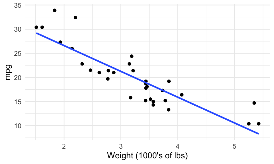

While you can plot a linear model using ggplot2’s geom_smooth() layer, you can’t really do much else in terms of the linear model, like inference. Because of this, we will explicitly fit linear models outside of ggplot.

Fitting a Model in R

Fitting a model in R typically involves using a function in the following format:

method(formula, data, options)

Method: A function such as:

Linear Regression: lm
Generalized Linear Regression: glm
Local regression: loess
Quantile regression: quantreg::rq
…

Formula: In R, takes the form y ~ x1 + x2 + ... + xp (use column names in your data frame), where y here means the outcome variable you’re interested in viewing in relation to other variables x1, x2, …

Data: The data frame or tibble. Can omit, if variables in the formula are defined in environment

Options: Specific to the method, and include ways to customize the model.

Running the code returns an object – usually a special type of list – that you can then work with to extract results.

For example, let’s fit a linear regression model on a car’s mileage per gallon (mpg, “Y” variable) from the car’s weight (wt, “X” variable). Notice that no special options are needed for lm().

my_lm <- lm(mpg ~ wt, data = mtcars)

my_lm


Call:
lm(formula = mpg ~ wt, data = mtcars)

Coefficients:
(Intercept)           wt  
     37.285       -5.344

Printing the model to the screen might lead you to incorrectly conclude that the model object my_lm only contains the above text. The reality is, my_lm contains a lot more, but special instructions have been given to R to only print out a special digested version of the object. This behaviour tends to be true with model objects in general, not just for lm(). Let’s

Summarizing the Model with `broom`

Now that you have the model object, there are typically three ways in which it’s useful to probe and use the model object. The broom package has three crown functions that make it easy to extract each piece of information by converting your model into a tibble:

tidy: extract statistical summaries about each “component” of the model.
augment: add columns to the original data frame containing predictions.
glance: extract statistical summaries about the model as a whole (a 1-row tibble).

`tidy()`

Use the tidy() function for a statistical summary of each component of your model, where each component gets a row in the output tibble. For lm(), tidy() gives one row per regression coefficient (slope and intercept).

tidy(my_lm)

# A tibble: 2 × 5
  term        estimate std.error statistic  p.value
  <chr>          <dbl>     <dbl>     <dbl>    <dbl>
1 (Intercept)    37.3      1.88      19.9  8.24e-19
2 wt             -5.34     0.559     -9.56 1.29e-10

tidy() only works if it makes sense to talk about model “components”.

`augment()`

Use the augment() function to make predictions on a dataset by augmenting predictions as a new column to your data. By default, augment() uses the dataset that was used to fit the model.

augment(my_lm) %>%
  print(n = 5)

# A tibble: 32 × 9
  .rownames           mpg    wt .fitted .resid   .hat .sigma  .cooksd .std.resid
  <chr>             <dbl> <dbl>   <dbl>  <dbl>  <dbl>  <dbl>    <dbl>      <dbl>
1 Mazda RX4          21    2.62    23.3 -2.28  0.0433   3.07  1.33e-2    -0.766 
2 Mazda RX4 Wag      21    2.88    21.9 -0.920 0.0352   3.09  1.72e-3    -0.307 
3 Datsun 710         22.8  2.32    24.9 -2.09  0.0584   3.07  1.54e-2    -0.706 
4 Hornet 4 Drive     21.4  3.22    20.1  1.30  0.0313   3.09  3.02e-3     0.433 
5 Hornet Sportabout  18.7  3.44    18.9 -0.200 0.0329   3.10  7.60e-5    -0.0668
# ℹ 27 more rows

We can also predict on new datasets. Here are predictions of mpg for cars weighing 3, 4, and 5 thousand lbs. In the following code, we make a predictor for wt = 3, 4, and 5.

augment(my_lm, newdata = tibble(wt = 3:5))

# A tibble: 3 × 2
     wt .fitted
  <int>   <dbl>
1     3    21.3
2     4    15.9
3     5    10.6

Notice that only the “X” variables are needed in the input tibble (wt), and that since the “Y” variable (mpg) wasn’t provided, augment() couldn’t calculate anything besides a prediction

`glance()`

Use the glance() function to extract a summary of the model as a whole, in the form of a one-row tibble. This will give you information related to the model fit.

glance(my_lm)

# A tibble: 1 × 12
  r.squared adj.r.squared sigma statistic  p.value    df logLik   AIC   BIC
      <dbl>         <dbl> <dbl>     <dbl>    <dbl> <dbl>  <dbl> <dbl> <dbl>
1     0.753         0.745  3.05      91.4 1.29e-10     1  -80.0  166.  170.
# ℹ 3 more variables: deviance <dbl>, df.residual <int>, nobs <int>

Summarizing the Model Without `broom`

In order for a model to work with the broom package, someone has to go out of their way to contribute to the broom package for that model. While this has happened for many common models, many others remain without broom compatibility.

Here’s how to work with these model objects in that case.

Prediction

If broom::augment() doesn’t work, then the developer of the model almost surely made it so that the predict() function works (not part of the broom package). The predict() function typically takes the same format of the augment() function, but usually doesn’t return a tibble.

Here are the first 5 predictions of mpg on the my_lm object, defaulting to predictions made on the original data:

predict(my_lm) %>% #do prediction on all values in the original dataset
  unname() %>% #remove colnames
  head(5) #look at first 5 values

[1] 23.28261 21.91977 24.88595 20.10265 18.90014

Here are the predictions of mpg made for cars with a weight of 3, 4, and 5 thousand lbs:

predict(my_lm, newdata = tibble(wt = 3:5)) %>% 
  unname()

[1] 21.25171 15.90724 10.56277

Checking the documentation of the predict() function for your model isn’t obvious, because the predict() function is a “generic” function. Your best bet is to append the model name after a dot. For example:

For a model fit with lm(), try ?predict.lm
For a model fit with rq(), try ?predict.rq (from the quantreg package)

If that doesn’t work, just google it: "Predict function for rq"

Inference

We can extract model information using summary() on the linear model:

summary(my_lm)


Call:
lm(formula = mpg ~ wt, data = mtcars)

Residuals:
    Min      1Q  Median      3Q     Max 
-4.5432 -2.3647 -0.1252  1.4096  6.8727 

Coefficients:
            Estimate Std. Error t value Pr(>|t|)    
(Intercept)  37.2851     1.8776  19.858  < 2e-16 ***
wt           -5.3445     0.5591  -9.559 1.29e-10 ***
---
Signif. codes:  0 '***' 0.001 '**' 0.01 '*' 0.05 '.' 0.1 ' ' 1

Residual standard error: 3.046 on 30 degrees of freedom
Multiple R-squared:  0.7528,    Adjusted R-squared:  0.7446 
F-statistic: 91.38 on 1 and 30 DF,  p-value: 1.294e-10

There’s a lot of information here. To extract a specific piece, we use $. For example,

summary(my_lm)$coefficients

             Estimate Std. Error   t value     Pr(>|t|)
(Intercept) 37.285126   1.877627 19.857575 8.241799e-19
wt          -5.344472   0.559101 -9.559044 1.293959e-10

This outputs a data frame of some of the model output regarding the regression coefficients. There are a ton of other items we can access, and to see them we can call names()

names(summary(my_lm))

 [1] "call"          "terms"         "residuals"     "coefficients" 
 [5] "aliased"       "sigma"         "df"            "r.squared"    
 [9] "adj.r.squared" "fstatistic"    "cov.unscaled"

For another example, wo see the adjusted R-squared valued of the model we can use

summary(my_lm)$adj.r.squared

[1] 0.7445939

Plotting Models in `ggplot2`

We can plot models (with one predictor/ X variable) using ggplot2 through the geom_smooth() layer. Specifying method="lm" gives us the linear regression fit (but only visually – very difficult to extract model components!):

ggplot(mtcars, aes(x = wt, y = mpg)) +
    geom_point() +
    geom_smooth(method = "lm", se = F) #se = F removes the confidence interval bands

`geom_smooth()` using formula = 'y ~ x'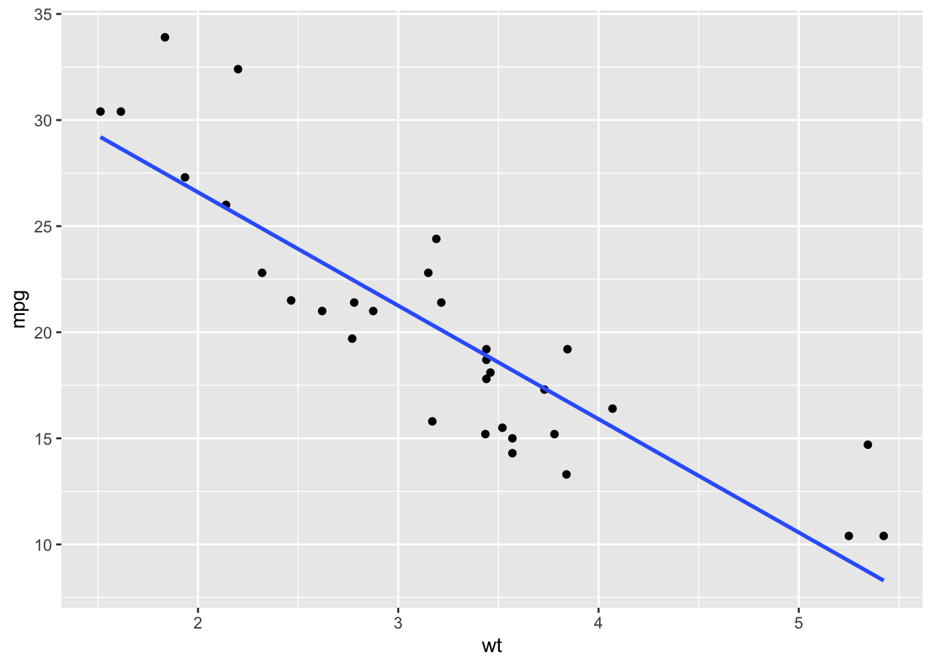

Example: `gapminder`

Let’s visualize some relationships in the gapminder dataset.

Let’s inspect Zimbabwe, which has a unique behavior in the lifeExp and year relationship.

gapminder_Zimbabwe <- gapminder %>% 
  filter(country == "Zimbabwe")

gapminder_Zimbabwe %>% 
  ggplot(aes(year, lifeExp)) + 
  geom_point() #add scatter plot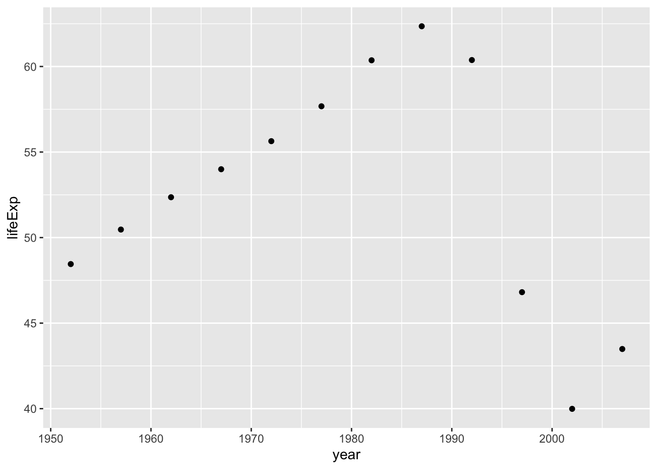

Now, let’s try fitting a linear model to this relationship

ggplot(gapminder_Zimbabwe, aes(year,lifeExp)) +
  geom_point() + #add the scatter plots
  geom_smooth(method = "lm", se = F) #add a linear regression line

`geom_smooth()` using formula = 'y ~ x'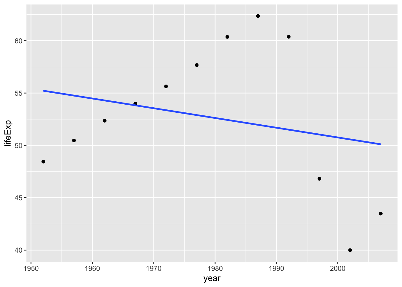

Not a great fit. Now we will try to fit a second degree polynomial and see what would that look like.

ggplot(gapminder_Zimbabwe, aes(year,lifeExp)) +
  geom_point() +
  geom_smooth(method = "lm",
              formula = y ~ poly(x,2), #second degree polynomial (quadratic)
              se = F)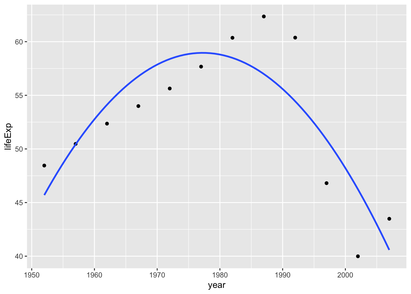

That’s a better fit. Visualizing data is a really good way to inform what types of models we should use in our analysis.

While this lecture only focused on two-dimensonal data (one y and one x), more sophisticaed statistical models can certainly handle more complexity and higher-dimensional data. If you’re interested, head to the Resources section at the end of this page to learn more.

Summary

function(formula, data, options) - most models in R follow this structure.
broom::augment() - uses a fitted model to obtain predictions. Puts this in a new column in existing tibble. Equivalent base-r function is predict().
broom::tidy() - used to extract statistical information on each component of a model. Equivalent is coef(summary(lm_object)).
broom::glance() - used to extract statistical summaries on the whole model. Always returns a 1-row tibble.
geom_smooth() - used to add geom_layer that shows a fitted line to the data. method and formula arguments can be used to customize model.

FEV Case study

While this is not a modelling class, let’s get a sense of where modelling would fit into a real data analysis by working through the final part of the FEV case study.

Worksheet A4

We will now spend some time attempting questions on the last part of Worksheet A4.

Resources

Video Lecture: The Model-Fitting Paradigm in R
The broom vignette
U Chicago Tutorial on model fitting in R (just the linear regression part).
An Introduction to Statistical Learning
Mike Marin’s R playlist on YouTube