3  Cross-validation concerns

In this document we study how to perform cross-validation when the model was selected or determined using the training data. Consider the following synthetic data set

dat <- read.table("data/fallacy.dat", header = TRUE, sep = ",")

This is the same data used in class. In this example we know what the “true” model is, and thus we also know what the “optimal” predictor is. However, let us ignore this knowledge, and build a linear model instead. Given how many variables are available, we use forward stepwise (AIC-based) to select a good subset of them to include in our linear model:

library(MASS)
p <- ncol(dat)
null <- lm(Y ~ 1, data = dat)
full <- lm(Y ~ ., data = dat) # needed for stepwise
step.lm <- stepAIC(null, scope = list(lower = null, upper = full), trace = FALSE)

Without thinking too much, we use 50 runs of 5-fold CV (ten runs) to compare the MSPE of the null model (which we know is “true”) and the one we obtained using forward stepwise:

n <- nrow(dat)
ii <- (1:n) %% 5 + 1
set.seed(17)
N <- 50
mspe.n <- mspe.st <- rep(0, N)
for (i in 1:N) {
  ii <- sample(ii)
  pr.n <- pr.st <- rep(0, n)
  for (j in 1:5) {
    tmp.st <- update(step.lm, data = dat[ii != j, ])
    pr.st[ii == j] <- predict(tmp.st, newdata = dat[ii == j, ])
    pr.n[ii == j] <- with(dat[ii != j, ], mean(Y))
  }
  mspe.st[i] <- with(dat, mean((Y - pr.st)^2))
  mspe.n[i] <- with(dat, mean((Y - pr.n)^2))
}
boxplot(mspe.st, mspe.n, names = c("Stepwise", "NULL"), col = c("gray60", "hotpink"), main = "Wrong")

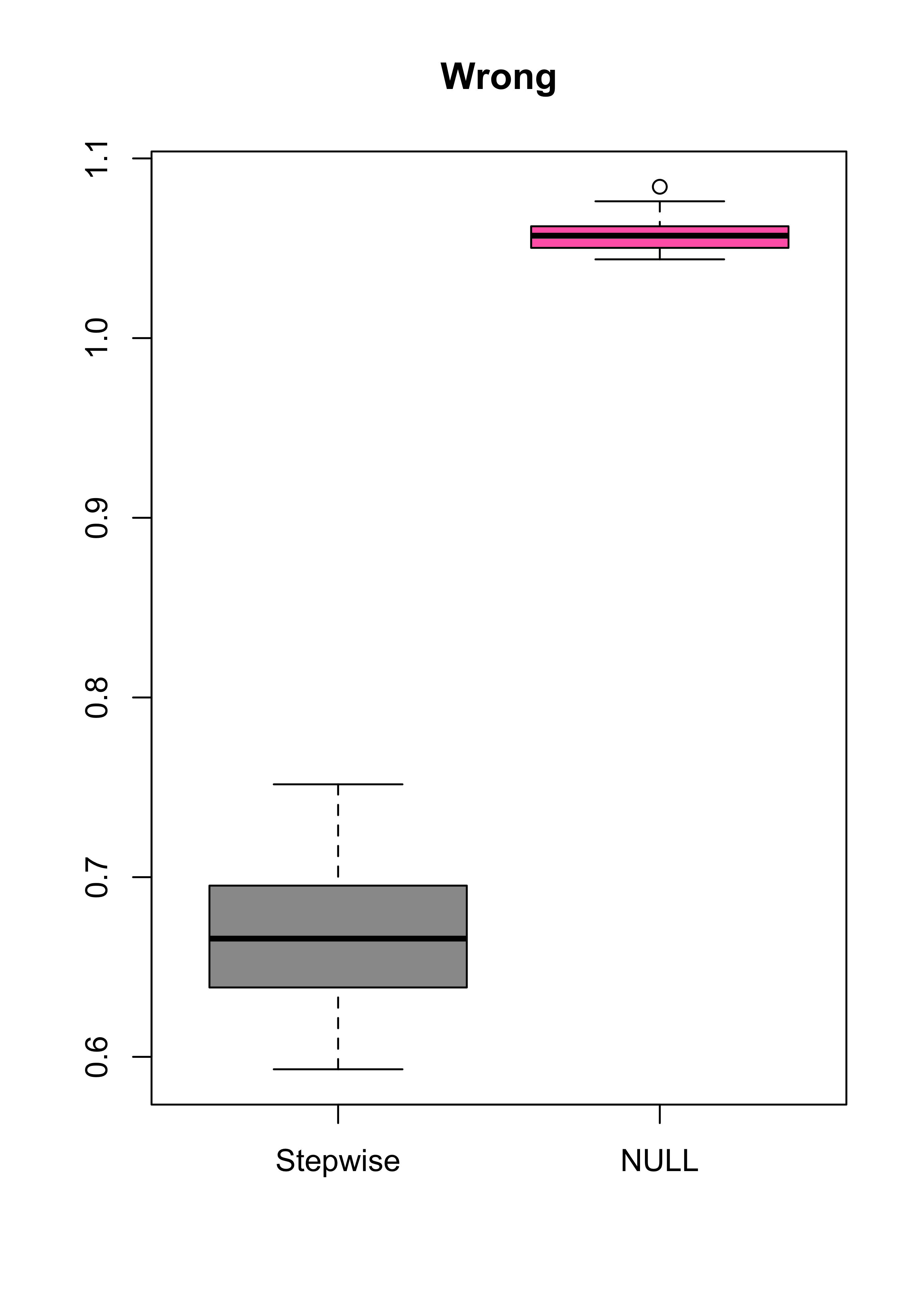
summary(mspe.st)
#>    Min. 1st Qu.  Median    Mean 3rd Qu.    Max. 
#>  0.5931  0.6392  0.6658  0.6663  0.6945  0.7517
summary(mspe.n)
#>    Min. 1st Qu.  Median    Mean 3rd Qu.    Max. 
#>   1.044   1.050   1.057   1.057   1.062   1.084

• Something is wrong! What? Why?
• What would you change above to obtain reliable estimates for the MSPE of the model selected with the stepwise approach?

3.1 Estimating MSPE with CV when the model was built using the data

Misuse of cross-validation is, unfortunately, not unusual. For one example see (Ambroise and McLachlan 2002).

In particular, for every fold one needs to repeat everything that was done with the training set (selecting variables, looking at pairwise correlations, AIC values, etc.)

3.2 Correlated covariates

Technological advances in recent decades have resulted in data being collected in a fundamentally different manner from the way it was done when most “classical” statistical methods were developed (early to mid 1900’s). Specifically, it is now not at all uncommon to have data sets with an abundance of potentially useful explanatory variables (for example with more variables than observations). Sometimes the investigators are not sure which of the collected variables can be expected to be useful or meaningful.

A consequence of this “wide net” data collection strategy is that many of the explanatory variables may be correlated with each other. In what follows we will illustrate some of the problems that this can cause both when training and interpreting models, and also with the resulting predictions.

3.2.1 Variables that were important may suddenly “dissappear”

Consider the air pollution data set we used earlier, and the reduced linear regression model discussed in class:

x <- read.table("data/rutgers-lib-30861_CSV-1.csv", header = TRUE, sep = ",")
reduced <- lm(MORT ~ POOR + HC + NOX + HOUS + NONW, data = x)
round(summary(reduced)$coef, 3)
#>             Estimate Std. Error t value Pr(>|t|)
#> (Intercept) 1172.831    143.241   8.188    0.000
#> POOR          -4.065      2.238  -1.817    0.075
#> HC            -1.480      0.333  -4.447    0.000
#> NOX            2.846      0.652   4.369    0.000
#> HOUS          -2.911      1.533  -1.899    0.063
#> NONW           4.470      0.846   5.283    0.000

Note that all coefficients seem to be significant based on the individual tests of hypothesis (with POOR and HOUS maybe only marginally so). In this sense all 5 explanatory varibles in this model appear to be relevant.

Now, we fit the full model, that is, we include all available explanatory variables in the data set:

full <- lm(MORT ~ ., data = x)
round(summary(full)$coef, 3)
#>             Estimate Std. Error t value Pr(>|t|)
#> (Intercept) 1763.981    437.327   4.034    0.000
#> PREC           1.905      0.924   2.063    0.045
#> JANT          -1.938      1.108  -1.748    0.087
#> JULT          -3.100      1.902  -1.630    0.110
#> OVR65         -9.065      8.486  -1.068    0.291
#> POPN        -106.826     69.780  -1.531    0.133
#> EDUC         -17.157     11.860  -1.447    0.155
#> HOUS          -0.651      1.768  -0.368    0.714
#> DENS           0.004      0.004   0.894    0.376
#> NONW           4.460      1.327   3.360    0.002
#> WWDRK         -0.187      1.662  -0.113    0.911
#> POOR          -0.168      3.227  -0.052    0.959
#> HC            -0.672      0.491  -1.369    0.178
#> NOX            1.340      1.006   1.333    0.190
#> SO.            0.086      0.148   0.585    0.562
#> HUMID          0.107      1.169   0.091    0.928

In the full model there are many more parameters that need to be estimated, and while two of them appear to be significantly different from zero (NONW and PREC), all the others appear to be redundant. In particular, note that the p-values for the individual test of hypotheses for 4 out of the 5 regression coefficients for the variables of the reduced model have now become not significant.

round(summary(full)$coef[names(coef(reduced)), ], 3)
#>             Estimate Std. Error t value Pr(>|t|)
#> (Intercept) 1763.981    437.327   4.034    0.000
#> POOR          -0.168      3.227  -0.052    0.959
#> HC            -0.672      0.491  -1.369    0.178
#> NOX            1.340      1.006   1.333    0.190
#> HOUS          -0.651      1.768  -0.368    0.714
#> NONW           4.460      1.327   3.360    0.002

In other words, the coeffficients of explanatory variables that appeared to be relevant in one model may turn to be “not significant” when other variables are included. This could pose some challenges for interpreting the estimated parameters of the models.

3.2.2 Why does this happen?

Recall that the covariance matrix of the least squares estimator involves the inverse of (X’X), where X’ denotes the transpose of the n x p matrix X (that contains each vector of explanatory variables as a row). It is easy to see that if two columns of X are linearly dependent, then X’X will be rank deficient. When two columns of X are “close” to being linearly dependent (e.g. their linear corrleation is high), then the matrix X’X will be ill-conditioned, and its inverse will have very large entries. This means that the estimated standard errors of the least squares estimator will be unduly large, resulting in non-significant test of hypotheses for each parameter separately, even if the global test for all of them simultaneously is highly significant.

3.2.3 Why is this a problem if we are interested in prediction?

Although in many applications one is interested in interpreting the parameters of the model, even if one is only trying to fit / train a model to do predictions, highly variable parameter estimators will typically result in a noticeable loss of prediction accuracy. This can be easily seen from the bias / variance factorization of the mean squared prediction error (MSPE) mentioned in class. Hence, better predictions can be obtained if one uses less-variable parameter (or regression function) estimators.

3.2.4 What can we do?

A commonly used strategy is to remove some explanatory variables from the model, leaving only non-redundant covariates. However, this is easier said than done. You will have seen some strategies in previous Statistics courses (e.g. stepwise variable selection). In coming weeks we will investigate other methods to deal with this problem.

Ambroise, Christophe, and Geoffrey J. McLachlan. 2002. “Selection Bias in Gene Extraction on the Basis of Microarray Gene-Expression Data.” Proceedings of the National Academy of Sciences 99 (10): 6562–66. https://doi.org/10.1073/pnas.102102699.