data(spam, package = "ElemStatLearn")
n <- nrow(spam)
set.seed(987)
ii <- sample(n, floor(n / 3))
spam.te <- spam[ii, ]
spam.tr <- spam[-ii, ]18 What is Adaboost doing, really?
Following the work of (Friedman, Hastie, and Tibshirani 2000) (see also Chapter 10 of [ESL]), we saw in class that Adaboost can be interpreted as fitting an additive model in a stepwise (greedy) way, using an exponential loss. It is then easy to prove that Adaboost.M1 is computing an approximation to the optimal classifier G( x ) = log[ P( Y = 1 | X = x ) / P( Y = -1 | X = x ) ] / 2, where optimal here is taken with respect to the exponential loss function. More specifically, Adaboost.M1 is using an additive model to approximate that function. In other words, Boosting is attempting to find functions \(f_1\), \(f_2\), …, \(f_N\) such that \(G(x) = \sum_i f_i( x^{(i)} )\), where \(x^{(i)}\) is a sub-vector of \(x\) (i.e. the function \(f_i\) only depends on some of the available features, typically a few of them: 1 or 2, say). Note that each \(f_i\) generally depends on a different subset of features than the other \(f_j\)’s.
Knowing the function the boosting algorithm is approximating (even if it does it in a greedy and suboptimal way), allows us to understand when the algorithm is expected to work well, and also when it may not work well. In particular, it provides one way to choose the complexity of the weak lerners used to construct the ensemble. For an example you can refer to the corresponding lab activity.
18.0.1 A more challenging example, the email spam data
The email spam data set is a relatively classic data set containing 57 features (potentially explanatory variables) measured on 4601 email messages. The goal is to predict whether an email is spam or not. The 57 features are a mix of continuous and discrete variables. More information can be found at https://archive.ics.uci.edu/ml/datasets/spambase.
We first load the data and randomly separate it into a training and a test set. A more thorough analysis would be to use full K-fold cross-validation, but given the computational complexity, I decided to leave the rest of this 3-fold CV exercise to the reader.
We now use Adaboost with 500 iterations, using stumps (1-split trees) as our weak learners / classifiers, and check the performance on the test set:
library(adabag)
onesplit <- rpart.control(cp = -1, maxdepth = 1, minsplit = 0, xval = 0)
bo1 <- boosting(spam ~ ., data = spam.tr, boos = FALSE, mfinal = 500, control = onesplit)
pr1 <- predict(bo1, newdata = spam.te)
table(spam.te$spam, pr1$class) # (pr1$confusion)
#>
#>         email spam
#>   email   883   39
#>   spam     45  566
The classification error rate on the test set is 0.055. We now compare it with that of a Random Forest and look at the fit:
library(randomForest)
set.seed(123)
(a <- randomForest(spam ~ ., data = spam.tr, ntree = 500))
#>
#> Call:
#>  randomForest(formula = spam ~ ., data = spam.tr, ntree = 500)
#>                Type of random forest: classification
#>                      Number of trees: 500
#> No. of variables tried at each split: 7
#>
#>         OOB estimate of  error rate: 5.05%
#> Confusion matrix:
#>       email spam class.error
#> email  1813   53  0.02840300
#> spam    102 1100  0.08485857
Note that the OOB estimate of the classification error rate is 0.051. The number of trees used seems to be appropriate in terms of the stability of the OOB error rate estimate:
plot(a)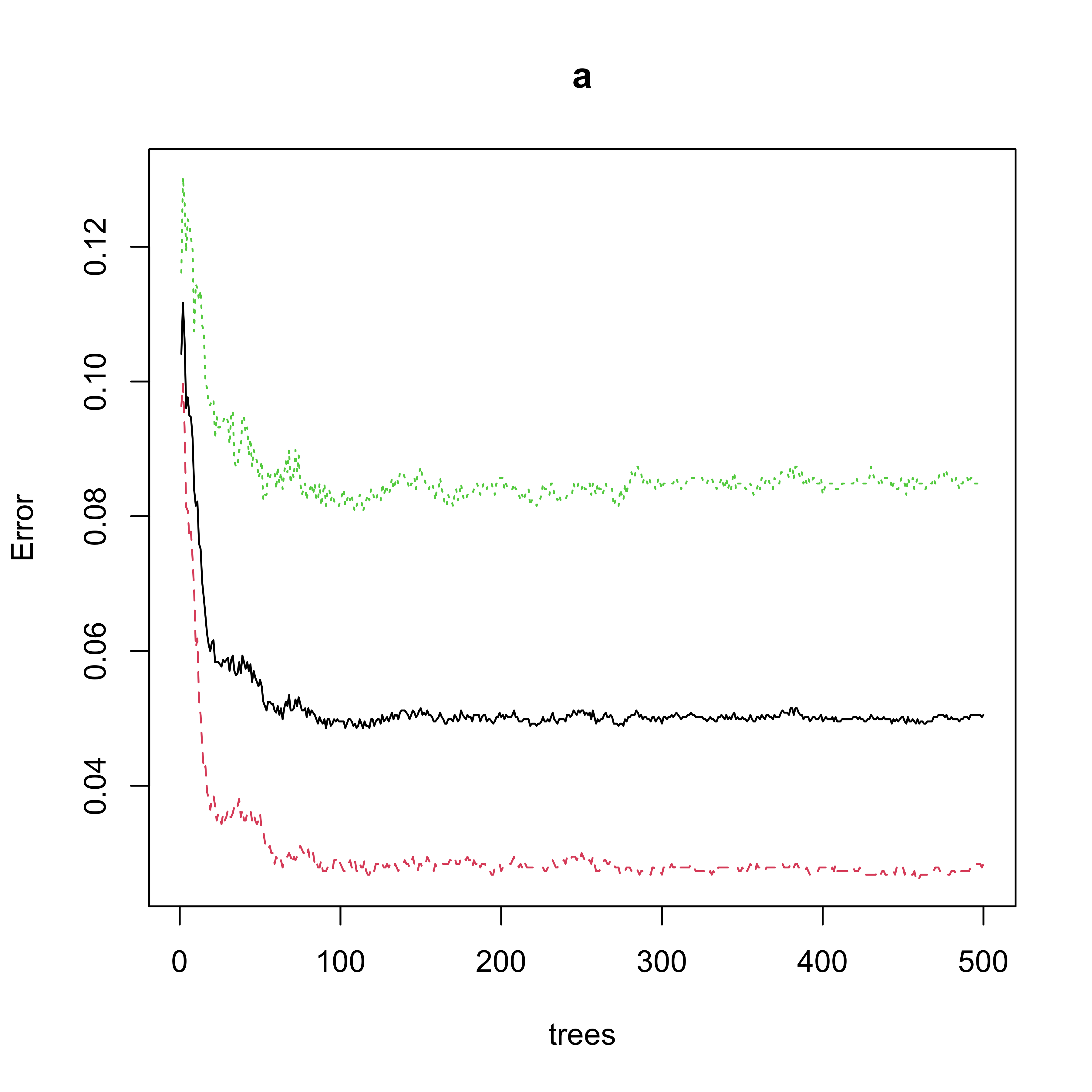
Now use the test set to estimate the error rate of the Random Forest (for a fair comparison with the one computed with boosting) and obtain
pr.rf <- predict(a, newdata = spam.te, type = "response")
table(spam.te$spam, pr.rf)
#>        pr.rf
#>         email spam
#>   email   886   36
#>   spam     36  575
The performance of Random Forests on this test set is better than that of boosting (recall that the estimated classification error rate for 1-split trees-based Adaboost was 0.055, while for the Random Forest is 0.047 on the test set and 0.051 using OOB).
Is there any room for improvement for Adaboost? As we discussed in class, depending on the interactions that may be present in the true classification function, we might be able to improve our boosting classifier by slightly increasing the complexity of our base ensemble members. Here we try to use 3-split classification trees, instead of the 1-split ones used above:
threesplits <- rpart.control(cp = -1, maxdepth = 3, minsplit = 0, xval = 0)
bo3 <- boosting(spam ~ ., data = spam.tr, boos = FALSE, mfinal = 500, control = threesplits)
pr3 <- predict(bo3, newdata = spam.te)
(pr3$confusion)
#>                Observed Class
#> Predicted Class email spam
#>           email   881   34
#>           spam     41  577
The number of elements on the boosting ensemble (500) appears to be appropriate when we look at the error rate on the test set as a function of the number of boosting iterations:
plot(errorevol(bo3, newdata = spam.te))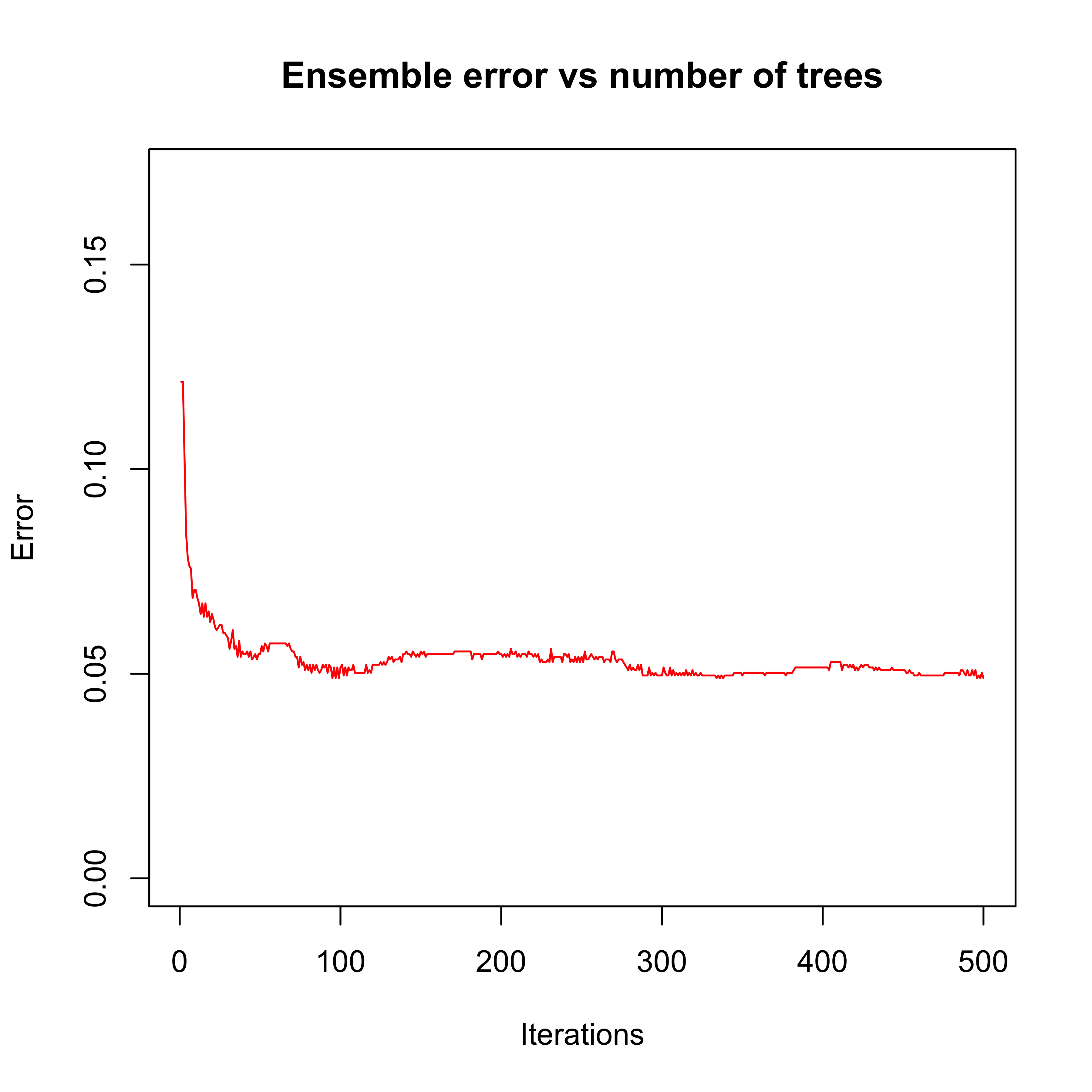
There is, in fact, a noticeable improvement in performance on this test set compared to the AdaBoost using stumps. The estimated classification error rate of AdaBoost using 3-split trees on this test set is 0.049. Recall that the estimated classification error rate for the Random Forest was 0.047 (or 0.051 using OOB).
As mentioned above you are strongly encouraged to finish this analysis by doing a complete K-fold CV analysis in order to compare boosting with random forests on these data.
18.0.2 An example on improving Adaboost’s performance including interactions
Some error I can’t track happens below
Consider the data set in the file boost.sim.csv. This is a synthetic data inspired by the well-known Boston Housing data. The response variable is class and the two predictors are lon and lat. We read the data set
sim <- read.table("data/boost.sim.csv", header = TRUE, sep = ",", row.names = 1)We split the data randomly into a training and a test set:
set.seed(123)
ii <- sample(nrow(sim), nrow(sim) / 3)
sim.tr <- sim[-ii, ]
sim.te <- sim[ii, ]
As before, we use stumps as our base classifiers
library(rpart)
stump <- rpart.control(cp = -1, maxdepth = 1, minsplit = 0, xval = 0)
and run 300 iterations of the boosting algorithm:
set.seed(17)
sim1 <- boosting(class ~ ., data = sim.tr, boos = FALSE, mfinal = 300, control = stump)
We examine the evolution of our ensemble on the test set:
plot(errorevol(sim1, newdata = sim.te))and note that the peformance is both disappointing and does not improve with the number of iterations. The error rate on the test set is . Based on the discussion in class about the effect of the complexity of the base classifiers, we now increase slightly their complexity: from stumps to trees with up to 2 splits:
twosplit <- rpart.control(cp = -1, maxdepth = 2, minsplit = 0, xval = 0)
set.seed(17)
sim2 <- boosting(class ~ ., data = sim.tr, boos = FALSE, mfinal = 300, control = twosplit)
plot(errorevol(sim2, newdata = sim.te))
Note that the error rate improves noticeably to . Interestingly, note as well that increasing the number of splits of the base classifiers does not seem to help much. With 3-split trees:
threesplit <- rpart.control(cp = -1, maxdepth = 3, minsplit = 0, xval = 0)
set.seed(17)
sim3 <- boosting(class ~ ., data = sim.tr, boos = FALSE, mfinal = 300, control = threesplit)
plot(errorevol(sim3, newdata = sim.te))
foursplit <- rpart.control(cp = -1, maxdepth = 4, minsplit = 0, xval = 0)
set.seed(17)
sim4 <- boosting(class ~ ., data = sim.tr, boos = FALSE, mfinal = 300, control = foursplit)the error rate on the test set is
round(predict(sim3, newdata = sim.te)$error, 4)while with 4-split trees the error rate is
round(predict(sim4, newdata = sim.te)$error, 4)The explanation for this is that the response variables in the data set were in fact generated through the following relationship:
log [ P ( Y = 1 | X = x ) / P ( Y = -1 | X = x ) ] / 2
 = [ max( x2 - 2, 0) - max( x1 + 1, 0) ] ( 1- x1 + x2 )
where \(x = (x_1, x_2)^\top\). Since stumps (1-split trees) are by definition functions of a single variable, boosting will not be able to approximate the above function using a linear combination of them, regardless of how many terms you use. Two-split trees, on the other hand, are able to model interactions between the two explanatory variables \(X_1\) (lon) and \(X_2\) (lat), and thus, with sufficient terms in the sum, we are able to approximate the above function relatively well.
As before, note that the analysis above may depend on the specific training / test split we used, so it is strongly suggested that you re-do it using a proper cross-validation setup.